ultrasphere

---

Documentation: https://ultrasphere.readthedocs.io

Source Code: https://github.com/ultrasphere-dev/ultrasphere

---

Vilenkin–Kuznetsov–Smorodinsky (VKS) polyspherical (hyperspherical) coordinates in NumPy / PyTorch

Installation

Install this via pip (or your favourite package manager):

pip install ultrasphere[plot]

Usage

Spherical Coordinates ↔ Cartesian Coordinates

First import the module and create a spherical coordinates object.

>>> import ultrasphere as us
>>> from array_api_compat import numpy as np
>>> from array_api_compat import torch
>>> rng = np.random.default_rng(0)
>>> c = us.create_spherical()

Getting spherical coordinates from cartesian coordinates:

>>> spherical = c.from_cartesian(torch.asarray([1.0, 2.0, 3.0]))
>>> spherical
{'r': tensor(3.7417), 'phi': tensor(1.1071), 'theta': tensor(0.6405)}

Getting cartesian coordinates from spherical coordinates:

>>> c.to_cartesian(spherical)
{0: tensor(1.), 1: tensor(2.0000), 2: tensor(3.)}

Using various VKS polyspherical coordinates

>>> us.create_polar()
SphericalCoordinates(a)
>>> us.create_spherical()
SphericalCoordinates(ba)
>>> us.create_standard(3)
SphericalCoordinates(bba)
>>> us.create_standard_prime(4)
SphericalCoordinates(b'b'b'a)
>>> us.create_hopf(3)
SphericalCoordinates(ccaacaa)
>>> us.create_from_branching_types("cbab'a")
SphericalCoordinates(cbab'a)
>>> us.create_random(10, rng=rng)
SphericalCoordinates(cacccaaaba)

One can convert between Cartesian coordinates and VKS polyspherical coordinates in the same way as above.

The name of the spherical nodes and cartesian nodes can be obtained by:

>>> c = us.create_standard(5)
>>> c.s_nodes
['theta0', 'theta1', 'theta2', 'theta3', 'theta4']
>>> c.s_ndim
5
>>> c.c_nodes
[0, 1, 2, 3, 4, 5]
>>> c.c_ndim
6

"r" is a special node which represents the radius and is not included in s_nodes.

The definition and notation of VKS polyspherical coordinates follows [Cohl2012, Appendix B]. Following sections would also help understand the VKS polyspherical coordinates.

• [Cohl2012] Cohl, H. (2012). Fourier, Gegenbauer and Jacobi Expansions for a Power-Law Fundamental Solution of the Polyharmonic Equation and Polyspherical Addition Theorems. Symmetry, Integrability and Geometry: Methods and Applications (SIGMA), 9. https://doi.org/10.3842/SIGMA.2013.042

Drawing spherical coordinates using rooted trees (Vilenkin's method of trees)

Python

>>> c = us.create_from_branching_types("ccabbab'b'ba")
>>> us.draw(c)
(6.5, 3.5)

CLI

ultrasphere "ccabbab'b'ba"

Output:

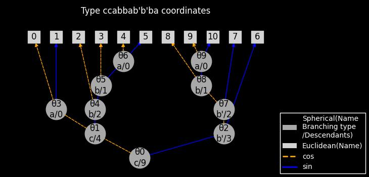
The image shows how Cartesian coordinates (leaf nodes) are calculated from spherical coordinates (internal nodes).

For example, $x_{10}$, corresponding to node 10, is a leaf node which ancestors are [θ0, θ2, θ7, θ8, θ9]. The edges which connect these nodes are named [sin, cos, cos, sin, sin], respectively. Thus, $x_{10}$ is calculated as:

$$ x_{10} = \sin \theta_0 \cos \theta_2 \cos \theta_7 \sin \theta_8 \sin \theta_9 $$

Integration over sphere using spherical coordinates

>>> c = us.create_spherical()
>>> f = lambda spherical: spherical["theta"] ** 2 * spherical["phi"]
>>> np.round(us.integrate(
...     c,
...     f,
...     False, # does not support separation of variables
...     10, # number of quadrature points
...     xp=np # the array namespace
... ), 5)
np.float64(110.02621)

Random sampling

Sampling random points uniformly from the unit ball:

>>> c = us.create_spherical()
>>> points_ball = us.random_ball(c, shape=(), xp=np, rng=rng)
>>> points_ball
array([0.12504754, 0.45095196, 0.32752147])
>>> np.linalg.vector_norm(points_ball)
np.float64(0.5711960026239531)

Sampling random points uniformly from the sphere (does not include interior points):

>>> points_sphere = us.random_ball(c, shape=(), xp=np, surface=True, rng=rng)
>>> points_sphere
array([-0.89670228, -0.44166441,  0.02928439])
>>> np.linalg.vector_norm(points_sphere)
np.float64(1.0)

References

• Barthe, F., Guédon, O., Mendelson, S., & Naor, A. (2005). A probabilistic approach to the geometry of the ? P n -ball. The Annals of Probability, 33. https://doi.org/10.1214/009117904000000874

Contributors ✨

Thanks goes to these wonderful people (emoji key):

This project follows the all-contributors specification. Contributions of any kind welcome!

Credits

This package was created with Copier and the browniebroke/pypackage-template project template.

The code examples in the documentation and docstrings are automatically tested as doctests using Sybil.