LAB 1

March 3, 2019

Object Classification

The purpose of this lab is to train a neural network using PyTorch on an image classification task. And get good results!

We are going to use a subset of Norb dataset for learning object classification. The dataset provided contains approximately 30K grayscale images of size 108 x 108. A sample snapshot of the images, as provided in the official webpage is shown below.

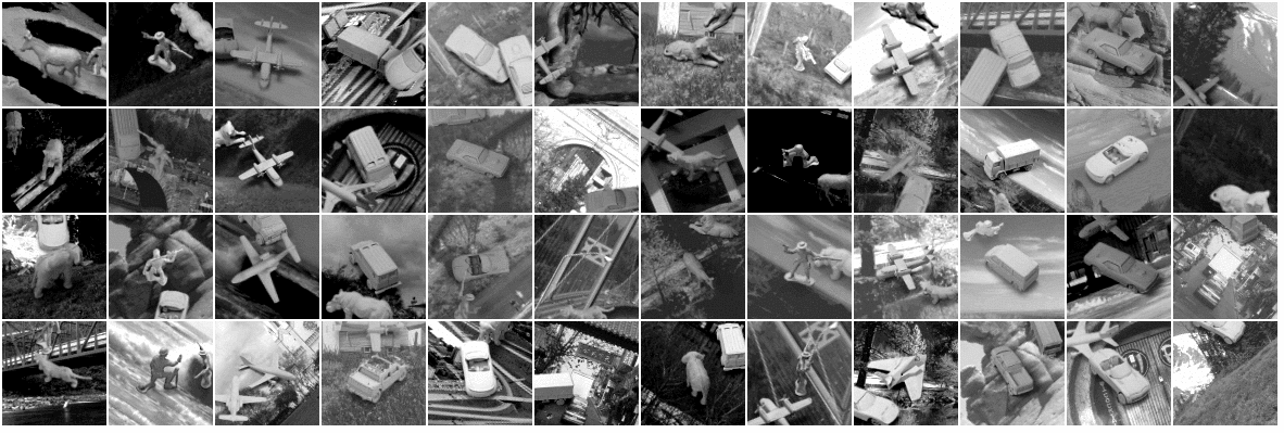
Zooming into the image, you should find different categories of images against complex backgrounds, and taken under different illumination conditions. There are six categories: humans, aircraft, four-legged animals, trucks, cars and, lastly, no-object.

Our data set has can be found in norb.tar.gz. The train.npy and test.npy contain the train and test images. The corresponding labels can be found in train_cat.npy and test_cat.npy files.

We also hope to compare the performance of a fully-connected network architecture against a Convolutional Neural Network architecture.

The implementation tasks for the assignment are divided into two parts:

1. Designing a network architecture using PyTorch’s nn module.
2. Training the designed network using PyTorch’s optim module.

Below you will find the details of tasks required for this assignment.

1. Fully-Connected Network: Write a function named create_fcn() in model.py file which returns a fully connected network variable. The network can be designed using nn.Sequential() container (refer to Sequential and Linear layer’s documentation). The network should have a series of Linear and ReLU layers with the output layer having as many neurons as the number of classes.
   
2. Criterion: Define the criterion in line number x. A criterion defines a loss function. In our case, use nn.CrossEntropyLoss() to define a cross entropy loss. We’ll use this variable later during optimization.
   
3. Optimizer: In the file train.py, we have defined a Stochastic Gradient Descent Optimizer. Fill-in the values of learning rate, momentum, weight decay, etc. You may also wish to experiment with other optimization functions like RMSProp, ADAM, etc which are provided by nn.optim package. Their documentation can be found in the this link.
   
4. Data Processing: The data, stored in dat.npy, contains images of toys captured from various angles. Each image has only one toy and the corresponding label of the images are stored in cat.npy. We have already set-up the data processing code for you. You may, optionally, want to play with the minibatch size or introduce noise to the data. You may also wish to preprocess the data differently. All this should be done in the functions preprocess_data() and add_noise() functions if you wish.
   
5. Experiments: Finally, test the networks on the given data. Train the networks for at least 10 epochs and observe the validation accuracy. You should be able to achieve at least 42% accuracy with a fully connected network.
   
6. Convolutional Neural Network: So far, we used nn.Sequential to construct our network. However, a Sequential container can be used only for simple networks since it restricts the network type. It is not usable in the case of, say, a Residual Network (ResNet) where the layers are not always stacked serially. To have more control over the network architecture, we’ll define a model class that implements PyTorch’s nn.Module superclass. We have provided a skeleton code in model.py file consisting of a simple CNN. The idea is simple: you need to write the forward() function which takes a variable x as input. As shown in the skeleton code, you may use __init__() function to initialize your layers and simply connect them the way you want in forward() function. You are free to design your custom network. Again, write a function named create_cnn() which returns a CNN model. This time, we need to use nn.Conv2d() and nn.MaxPool2d() functions. After stacking multiple Conv-ReLU-MaxPool layers, flatten out the activation using torch.View() and feed them to a fully connected layer that outputs the class probabilities.

For your CNN model, make appropriate changes in the train_cnn.py file. Once done, train this network. You should be able to see a significant improvement in performance (45% vs 75%).