In today's digital landscape, the ability to efficiently and accurately capture high volumes of network traffic is critical for a variety of domains, including cybersecurity, network optimization, and high-frequency trading (HFT). High-rate packet capture systems are designed to address the challenges of processing and storing immense quantities of network packet data with minimal latency and error. These systems play a vital role in maintaining the integrity, performance, and security of modern networks.
This project explores the development of a robust high-rate packet capture system, delving into the underlying technologies, methodologies, and challenges associated with high-speed data acquisition. The integration of advanced hardware configurations, optimized software solutions, and precision timing mechanisms aims to meet the stringent requirements of ultra-low latency (ULL) environments, particularly those critical to HFT operations.
Through this report, I examine the foundational principles of packet-switching networks, the architectural considerations for ULL data processing, and the practical applications of packet capture systems in industries where nanoseconds can define success or failure. Additionally, I address the technical and operational hurdles involved in implementing such systems, including efficient data storage, error handling, and scalability.
This report contributes to the advancement of high-rate packet capture technologies by bridging theoretical insights with practical implementations, paving the way for enhanced network performance and strategic decision-making in real-time data-driven environments.
- Emails:
- University: [email protected]
- Personal: [email protected]
- Websites:
- Personality research
- Guided by University of Illinois at Urbana-Champaign Professor, Dr. Brent Roberts
- The OSI Model
- Packets and Networks
- Time Synchronization
- Specific use cases for packet capture
- HFT setup
- Exchange and trading firm architecture
- Co-location (traders and exchanges in the same exchanges)
- Synchronization of clocks across data centers
- Backtesting with historical data
- Electronic exchange architecture
- Regulatory Requirements: MiFID II
- Why do financial trading firms capture network data?
- Primary types of data used by HFT firms
- Electrical characteristics of network technologies
- Anecdote: challenges in capturing high-speed data
- Challenges in packet capture for ULL environments
- Challenges in packet capture for ULL environments
- Methods of packet capture
- Recording packets on a computer
- Clocks and timestamping
- Issues and optimization in packet capture
- Specialized packet capture techniques
- Difficulties of writing A LOT of data
- Specialized devices (besides AMD's Solarflare/Xilinix devices)
- Packet recording formats
- Methods of configuring a NIC
- Computer architecture: PCIe bus, NICs, and the use of various NICs
- SolarCapture
- Storage
The Open Systems Interconnection (OSI) Model (also known as the OSI Reference Model), is an example of a reference model which conceptualizes standard communication functions of a telecommunications or computing system without focusing on its underlying internal structure and technology. It is a cornerstone in the field of networking as it simplifies the troubleshooting tasks as it helps to break down a problem and narrowing it down to one or more layers of the OSI model, thus avoiding a lot of unnecessary work, especially in identifying the origin of attacks, exploits, bugs, and other network issues.
The OSI Model was developed starting in the late 1970s to support the emergence of the diverse computer networking methods that competed to be in the large national networking efforts in France, the United Kingdom, and the United States. In the 1980s, the OSI Model became a working product of the Open Systems Interconnection group at the International Organization for Standardization (ISO).
The OSI Model is often memorized with the following mnemonic: "Please Do Not Throw Sausage Pizza Away", which stands for:
- Please - Physical Layer
- Do - Data Link Layer
- Not - Network Layer
- Throw - Transport Layer
- Sausage - Session Layer
- Pizza - Presentation Layer
- Away - Application Layer
Both the name (e.g. Session Layer) and number (e.g. Layer 5) are used interchangeably.
Starting from the Application layer working through each layer, the layers are defined as follows:
-
The Application layer (Layer 7) is the top-most layer of the OSI model and serves as the interface between the end-user applications and the network. It interacts with the operating system or application whenever the user chooses to transfer files, read messages, or perform other network-related activities (e.g., visit a website). These applications call the lower layers to fetch and deliver their data.
Common protocols that operate at the Application layer include:
- HyperText Transfer Protocol (HTTP)
- File Transfer Protocol (FTP)
- Simple Mail Transfer Protocol (SMTP)
-
The Presentation layer (Layer 6) is responsible for data representation and encryption and takes data provided by the Application layer and converts it into a standard format that the other layers can understand.
Common tasks at the presentation layer include:
- Data encryption and decryption
- Reformatting
- Compression and decompression
Common protocols and standards that operate at the Presentation layer include:
- Secure Sockets Layer (SSL)
- Transport Layer Security (TLS)
- American Standard Code for Information Interchange (ASCII)
- Joint Photographic Experts Group (JPEG)
-
The Session layer (Layer 5) is responsible for inter-host communication and establishes, maintains, and terminates user connections.
Common protocols that operate at the Session layer include:
- Network Basic Input/Output System (NetBIOS)
- Server Message Block (SMB)
-
The Transport layer (Layer 4) is responsible for end-to-end connections and connection reliability.
Overall, the Transport layer is responsible for:
- Detecting and correcting connection-related errors
- Controlling the flow of data
- Sequencing data
- Determining the size of a packet, also known as a datagram.
When sending data, the Transport layer may break the received data into smaller pieces (called segments) for transmission, and uniquely number them. When receiving data, the Transport layer is responsible for making sure the data arrives intact (not damaged) and then putting everything together in its original order before handing the data off to the Session layer.
Common protocols that operate at the Transport layer include:
- Transmission Control Protocol (TCP)
- User Datagram Protocol (UDP)
-
The Network layer (layer 3) is responsible for path determination and IP and is responsible for tasks such as:
- Delivering packets
- Providing logical addressing (e.g., Internet Protocol (IP) addresses)
- Determining the best path for a packet
A communications session does not necessarily always occur between two systems on the same network. Sometimes, those systems are literally half a world away from each other. In such cases, the Network layer contains the mechanisms that map out the best route (or path) a data packet can travel on a network. The route includes every device that handles the packet between its source to its destination, including routers, switches, and firewalls, for that session.
Common protocols that operate at the Network layer include:
- Internet Protocol version 4 (IPv4) and version 6 (IPv6)
- Internet Control Message Protocol version 4 (ICMPv4) and version 6 (ICMPv6)
Common hardware that operates at the Network layer includes:
- Routers
- Layer 3 switches
-
The Data Link layer (Layer 6) is responsible for Media Access Control (MAC) and logical link control (LLC) (physical addressing) and is where the rules, processes, and mechanisms for sending and receiving data are over a local area network (LAN) are defined.
Common tasks the Data Link layer is responsible for include:
- Accessing the transmission media
- Hardware addressing
- Detecting Data Link-related errors
- Controlling the flow of frames, which are the basic packaging for LAN traffic as it travels across the medium.
A common protocol that operates on the Data Link layer is the Address Resolution Protocol (ARP).
Common hardware that operates at the Data Link layer includes:
- Bridges, which are devices that connect two network segments by analyzing incoming frames and making decisions about where to direct them based on each frame's address.
- Switches, which are essentially high-speed, multi-port bridges; a port is an opening on computer networking equipment that cables plug into. Their purpose is to connect wired hardware in a LAN to one another to share data.
- Network interface cards (NICs), which are computer hardware that connects to computer to a computer network. It plugs into an expansion slot or is integrated on the motherboard and allows systems to communicate over a network, either by using cables or wirelessly.
-
The Physical layer (Layer 7) is responsible for media, signal, and binary transmission and it includes all the procedures and mechanisms needed to both place data onto the network's medium for transmission and to receive the data sent to your system on that same medium. For example, bits are converted into electrical or light impulses through a process known as encoding, a process which often occurs at the Physical layer through some transmission medium.
Common hardware and standards that operate at the Physical layer include:
- Cabling
- Repeaters, which regenerate a signal before it becomes unreadable due to transmission power loss and extends a network's reach.
- Modems
- Adapter cards
- Physical standards
- IEEE 802.3 (Ethernet)
- IEEE 802.11 (Wireless)
While the OSI Model is a widely recognized framework for understanding network communications, it has also faced (valid) criticisms over the years. Some of these criticisms include:
-
Lack of implementation: Although the OSI model was developed as a theoretical framework to standardize network communication, it has not been widely implemented in practice.
Instead, the TCP/IP model is the de facto standard for networking.
-
Limited practicality: The OSI Model was designed to be a general-purpose communication system, but it did not fully consider the practical needs of real-world networks.
As a result, the OSI Model is often criticized for being overly theoretical and not addressing the practical concerns of network engineers and administrators. For example, there's no Session nor Presentation layers in modern networks. The concepts exist, but not as layers and not with the functionality those layers envisioned.
For example, the Session layer wanted "synchronization points" to synchronize transactions. This model never worked, not to mention how the synchronization works on the Internet is vastly more complex, with most organizations designing their own implementations.
-
Lack of flexibility: The OSI Model is often criticized for being inflexible and not adaptable to new technologies or emerging trends.
As a result, the OSI Model has not kept pace with the rapid changes in networking technologies and the increasing demand for more flexible and dynamic network designs and architectures.
A packet, also known as a datagram, acts as an envelope for Transmission Control Protocol (TCP) and User Datagram Protocol (UDP) data. Packets contain information necessary for routers to transfer data between different local area network (LAN) segments (dividing one LAN into parts, with each part called a LAN Segment) over a packet-switched network. Similar to a real-life package, each network packet includes control data and user data being transferred. Control data, also known as the header, includes data for delivering the payload, such as the source and destination network addresses; error detection codes; and sequencing information, and is used by networking hardware to direct the packet to its destination and ensure data integrity. User data, also known as the payload, is data that is carried on behalf of an application. The payload is extracted and used by an operation system, application software, or higher layer protocols.
Network packets are crucial because they enable the efficient and reliable transfer of data over complex networks. Instead of sending large files or streams of data as a single, continuous block—which could monopolize network resources and be more susceptible to errors—data is broken into smaller, manageable pieces. These packets can then be transmitted independently and reassembled at the destination, allowing for better utilization of network bandwidth and resources. Often, when a user sends a file across a network, it gets transferred in smaller data packets, not in one piece. For example, a 5MB file will be divided into some number of packets (e.g., 3), each with a source and destination address (e.g., Source and Destination IP Addresses), the number of packets in the entire data file (3), and the sequence number so the packets can be reassembled at their destination once they have all been received (e.g., "hey receiver, this is packet 1 of 3").
While crucial as a data structure structure, packets need a routing mechanism to ensure proper network communications. Packet-switching, is one such mechanism, where packets have a fundamental role. Packet-switching is known as a method of grouping data into packets that are transmitted over a digital network and refers to the routing and transferring of data by means of addressed packets so that a channel is occupied during the transmission of the packet only, and upon completion of the transmission, the channel is made available for the transfer of other traffic. This means that packets can take different paths to reach the same destination, optimizing efficiency and reliability.
Packet-switched networks are:
-
Efficient:
Packets can be routed through the least congested paths, making optimal use of bandwidth.
-
Reliable:
If a particular path fails or becomes congested, packets can be rerouted through alternative paths.
-
Scalable:
Networks can be easily accommodate growth, as packets find the best available routes without the need for dedicated circuits.
Thus, packet-switched networks contrast with circuit-switched networks, where a dedicated communication path is established between two endpoints for the duration of the session (e.g., traditional telephone networks). Packet-switching is more flexible and efficient for data transmission, making it the primary basis for data communications in computer networks worldwide. In regard to HFT, the ubiquitousness of packet-switched networks give credibility to their flexibility and efficiency to provide HFT firms the ability to route data efficiently and to adapt to network conditions. This efficiency and adaptability of packet-switched networks ensures that orders, trades, and market data updates are transmitted with minimal latency, enabled by ultra-low latency (ULL) switches. As a result, packet-switched networks with ULL switches improve the competitiveness and profitability of trading strategies, as the ultra timely information can lead to better decision-making and faster execution.
A packet includes 3 components:
- A header, with control information, such as the source address of the sending host; the destination address of the receiving host; the length of the packet (in bytes); the sequencing (or proper ordering) of the individual packets; and the type of data being carried by the packet (e.g., Layer 7 application data).
- The data/body/payload: includes the data that is carried on behalf of an application.
- The trailer/footer: provides mechanisms for detecting errors during transmission and correcting them, along with information to verify the packet’s contents (e.g., Cyclic Redundancy Check (CRC)).
To easily conceptualize a packet, the idea of a postal letter is frequently used:
- The header is like the envelope
- The payload is the entire content(s) inside the envelope (e.g., a love letter), and
- The footer is your signature at the bottom of the love letter.
Packets operate at Layer 3 (the Network Layer) of the OSI Model:
- From the sender's perspective, data moves down the layers of OSI model, with each layer adding header or trailer information.
- Data travels up layers at the receiving system, with each layer removing the header or trailer information placed by the corresponding sender layer.
A packet can also be created using various software, also known as packet crafting tools (e.g., Scapy, hping, Nmap).
There are various types of packets but a few of them are most important for HFT firms.

Ethernet II frames are the most popular frame type used today, operate at the Data Link layer (Layer 2) of the OSI model, are used within LANs.
The core structure of an Ethernet frame consists of 7 fields:
- Preamble (7 bytes): A sequence of alternating 1s and 0s used to synchronize the receivers on the network before the actual data arrives; it allows devices to prepare for the reception of a frame.
- Start Frame Delimiter (SFD) (1 byte): Indicates the start of the frame and helps align the data bits properly.
- Destination MAC Address (part of the frame Header) (6 bytes): The physical hardware address of the Network Interface Card (NIC) to which the frame is being sent.
- Source MAC Address (part of the frame Header) (6 bytes): The physical hardware address of the NIC from which the message originated.
- Frame Type(2 bytes) (part of the frame Header): Specifies the type of higher layer protocol data that follows the header in the data portion of the Ethernet frame (e.g., 0x0806 in this field means ARP data follows next in the Data portion of the frame).
- Data/Payload (46 - 1500 bytes): Contains the encapsulated data, such as an IP packet or other higher-layer data. The minimum size ensures proper collision detection.
- Frame Check Sequence (FCS) (4 bytes): A Cyclic Redundancy Check (CRC) value used for error detection to ensure data integrity.
To summarize, Ethernet frames encapsulate data for transmission over the physical medium. They handle addressing within the LAN and ensure that data is delivered to the correct device. The FCS helps detect any errors that may have occurred during transmission, prompting retransmission if necessary. In HFT environments, any delay or error in data transmission can lead to missed trading opportunities or financial losses. Network engineers in HFT firms focus on optimizing Ethernet frame handling by minimizing Ethernet collisions, reducing latency through ULL switches, and ensuring that hardware components are capable of handling the required data rates (e.g. 100 Mbps to 100 Gbps, depending on the Ethernet cable standard used).
IP packets operate at Layer 3 (the Network Layer) and are responsible for routing data across interconnected networks, such as the Internet. IP packets, also known as IP datagrams, act as an envelope for TCP, UDP, and higher-layer protocol data/information (e.g., a webpage request). The IP packets contain logical addressing information (e.g., source/destination IP addresses) necessary for hosts to transfer the packets between different network segments.
There are two main Internet Protocols: Internet Protocol version 4 (IPv4) and Internet Protocol version 6 (IPv6).
-
IPv4 Header Structure
 IPv4 Header Structure.
Source: Matt BaxterSpecified in RFC 791, IPv4 is a connectionless protocol where each packet is treated independently than the others. An IPv4 packet has the following structure:
-
Version (4 bits): Identifies the version of IP (e.g. v4 or v6) used to generate the datagram.
The purpose of this field is to ensure compatibility between devices that may be running different versions of the IP (a dual-stack system is one running both versions of IPv4 and IPv6 software).
-
Header Length (4 bits): Specifies the length of the IP header for the packet.
The Header length is important to help the receiving host determine where in the IP datagram the data actually starts (the data portion of a packet starts immediately after the IP header ends). The numerical value found in this field is shown as a multiplier of 4 bytes (e.g., a value of 5 in this field means the IP header length is 20 bytes total (
$5\ x\ 4 = 20$ )). The maximum value in this field is 15 (or 60 bytes). -
Type of Service (ToS) (8 bits): Defines the priority and the Quality of Service (QoS) parameters for the packet.
This field is now now referred to as Differentiated Services (DiffServ) and Explicit Congestion Notification (ECN).
The updated DiffServ field allows for up to 64 values and a greater range of packet-forwarding behaviors (i.e. per-hop behaviors (PHBs)). DiffServ is defined a Class of Service (CoS) which engages in traffic classification, a more scalable and flexible approach than QoS since DiffServ allocates network resources on a per-class basis and sophisticated network operations only need to be implemented at network boundaries or hosts. Marking a packet with a high Differentiated Services Code Point (DSCP) value gives the packet an Expedited Forwarding (EF) group treatment, which is suited for traffic with strict QoS requirements for latency, packet loss, and jitter (Sources: https://www.techtarget.com/whatis/definition/Differentiated-Services-DiffServ-or-DS, https://www.cisco.com/c/en/us/products/ios-nx-os-software/differentiated-services/index.html)
ECN enables end-to-end congestion notification between two endpoints on TCP/IP based networks. ECN notifies networks about congestion with the goal of reducing packet loss and delay by making the sending device decrease the transmission rate until the congestion clears, without dropping packets. (Source: https://www.juniper.net/documentation/us/en/software/junos/cos/topics/concept/cos-qfx-series-explicit-congestion-notification-understanding.html)
-
Total Length (16 bits): Identifies he total length of the IP datagram, including the header and data (in bytes).
The value in this field cannot exceed 65,535 bytes (if the field is 16 bits in length, that means
$2^{16}$ is the largest possible value, but since the first possible value is 0, the maximum value is$2^{16}$ - 1, or 65,535). -
Identification (16 bits): Used for uniquely identifying the group of fragments of a single IP datagram.
This field (and the next two: Flags and Fragment Offset) ensure data is rebuilt on the receiving end properly. IP can break a packet it receives from a higher-level protocol into smaller packets (A.K.A. fragments), depending on the maximum size of the packet supported by the underlying network transmission technology. On the receiving end, these packets need to be reassembled.
-
Flags (3 bits): Signifies fragmentation options (e.g., whether or not fragments are allowed).
The sender can also use this field to tell the receiving host that more fragments are on the way (which is done with the More Fragments (MF) flag).
-
Fragmented Offset (13 bits): Identifies where the datagram fragment belongs in the incoming set of fragments by assigning a number to each one (known as the offset).
The receiving host will then use these numbers to reassemble the data correctly. This field is measured in units of 8-byte blocks. For example, a value of 2 in this field means to place the data 16 bytes into the packet when it's reassembled. This allows a maximum offset value of 65,528. The first fragment has an offset value of 0. This field is only applicable if fragments are allowed/set.
-
Time to Live (TTL) (8 bits): Sets an upper limit on the number of routers through which a datagram can pass to prevent it from circulating indefinitely.
The initial TTL value is set as a system default in the tCP/IP stack implementation of the various OS vendors, where each OS uses its own unique TTL value. Each router that handles an IP datagram is required to decrement the TTL value by 1. When the TTL value reaches 0, the datagram is discarded, and the sender is notified with an error message. This error message when TTL reaches 0 prevents packets from getting caught in loops forever (a routing loop happens when a data packet is continually routed through the same routers over and over, never reaching their destination).
-
Protocol (8 bits): Indicates the protocol that follows the IPv4 header (e.g., ICMP, TCP, UDP).
-
Header Checksum (16 bits): Contains a computed value used by the receiving host to ensure the integrity of the header information of the packet.
-
Source IP Address (32 bits): A.K.A. the Network Layer Address, it specifies the IPv4 address of the sending host.
-
Destination IP Address (32 bits): Specifies the recipient of the packet.
-
Options (variable length): Contains additional header options, such as optional routing and timing information.
-
-
IPv4 Data
What follows the IPv4 header is the data portion of the packet, which encapsulates the original application data sent by the source host, plus information added by any other layers (e.g. TCP, UDP). The size of the data portion of a packet varies in length.
-
IPv6 Features and Differences from IPv4
Like IPv4, IPv6 operates at Layer 3 (the Network Layer) of the OSI model; however, IPv6 has many features that improve on and differentiate it from IPv4:
-
Most transport- and application-layer protocols need little or no change to operate over IPv6. Exceptions are application protocols that embed network-layer addresses (e.g., FTP, Network Time Protocol (NTPv3)).
-
IPv6 specifies a new packet format, designed to minimize packet-header processing.
Since headers of the IPv4 packets and IPv6 packets ar significantly different, the 2 protocols are not interoperable.
-
IPv6 has a larger address space
The Size of an IPv6 address is 128 bits (
$2^{128}$ or$3.4\ x\ 10^{38}$ possible addresses), compared to 32 bits in IPv4 ($2^{32}$ possible addresses). The longer addresses allow for a systematic and hierarchical allocation of addresses and efficient route aggregation. -
Auto-configuration
IPv6 hosts can configure themselves automatically with help from a router on the local link, or dynamically via a DHCPv6 server.
-
Multicast
Multicast is part of the base specification of IPv6, unlike in IPv4, where multicast is optional, although usually implemented.
-
Broadcast
IPv6 does not implement broadcast. Instead IPv6 treats broadcasts as a special cast of multicasting.
-
Mandatory Network-Layer Security
Internet Protocol Security (IPSec), the protocol for IP encryption and authentication, forms an integral part of the base protocol suite in IPv6.
-
Simplified Processing by Routers
A number of simplifications have been made to the IPv6 packet header. The process of packet forwarding has also been simplified to make packet processing by routers simpler and more efficient (the IPv4 header was inefficient because routing required the analysis of each IPv4 header field).
- The IPv6 header is not protected by a checksum. Instead, integrity protection is assumed to be assured by a transport layer checksum.
- The TTL field of IPv4 has been renamed to Hop Limit, reflecting the fact that routers are no longer expected to compute the time a packet has spent in a queue.
-
The size of the IPv6 header has doubled (from 20 bytes for a minimum-sized IPv4 header) to 40 bytes.
 IPv6 Header Structure.
Source: Matt Baxter
An IPv6 packet is composed of the following parts:
- Mandatory Base Header (40 bytes).
- Followed by the payload (up to 65,535 bytes), which includes optional IPv6 Extension Headers and data from upper layer protocols.
-
-
IPv6 Base Header Structure
 IPv6 Base Structure.
Designed for routing efficiency, the IPv6 base header has the following fields:
-
Version (4 bits): Just like IPv4, identifies the version of IP used to generate the datagram.
This field ensures compatibility between systems that may be running different versions of the Internet Protocol.
-
Traffic Class (8 bits): Defines the priority of the packet with respect to other packets from the same source. For example, if 1 of 2 consecutive datagrams must be discarded due to congestion, the datagram with the lower packet priority will be discarded.
IPv6 divides traffic into 2 broad categories:
- Congestion-controlled, and
- Non-congestion controlled
Congestion-controlled traffic has the source adapt itself to the traffic slowdown. In this type of traffic, it is understood that packets may arrive delayed, lost, or received out of order. Congestion-controlled data are assigned priorities from 0-7, with 0 being the lowest (no priority set) and 7 the highest (control traffic).
Non-congestion controlled traffic refers to the type of traffic that expects minimum delay. Discarding the packet(s) is not desireable and retransmission, in most cases, is impossible. Thus, the source does not adapt itself to congestion. Real-time audio and video are examples of this type of traffic. Priority numbers from 8-15 are assigned to this type of traffic. Generally speaking, data containing less redundancy (e.g., low fidelity audio or video) can be given a higher priority (15); data containing more redundancy (e.g., high-fidelity audio and video) are given a lower priority (8).
-
Flow Label (20 bits): Designed to provide special handling for a particular flow of data.
A sequence of packets, sent from a particular source to a particular destination, that needs special handling by routers is called a flow of packets. The combination of the source address and the value of the flow label uniquely defines a flow of packets. To a router, a flow is a sequence of packets that share the same characteristics (e.g., traveling the same path, using the same resources, having the same kind of security requirements, etc.). In its simplest form, a flow label can be used to speed up the processing of a packet by a router (e.g., when a router receives a packet, instead of consulting the routing table and going through a routing algorithm to define the address of the next hop, it can easily look in a flow label table for the next hop).
In its more sophisticated form, a flow label can be used to support the transmission of a real-time audio and video. Real-time audio or video, in digital form, require resources (e.g., high bandwidth, large buffers, long processing time). A process can make a reservation for these resources beforehand to guarantee that real-time data will not be delayed due to a lack of resources. The use of real-time data and the reservation of these resources require other protocols (e.g., Real-Time Protocol (RTP), Resource Reservation Protocol (RSVP)).
-
Payload Length (16 bits): Defines the length of the data portion of the IPv6 datagram.
This field includes the optional extension headers and any upper-layer data. Using the 16 bits, an IPv6 payload of up to 65,535 bytes can be indicated. For payload lengths greater than 65,535 bytes, the Payload Length field is set to 0 and the Jumbo Payload option is used in the Hop-by-Hop Options extension header, which is briefly described in the IPv6 Extension Headers section.
-
Next Header (8 bits): Defines the payload that follows the base header in the datagram (similar to the Protocol field in IPv4).
It is either one of the option extension headers used by IP, or the header of an encapsulated packet (e.g., UDP, TCP, ICMP).
-
Hop Limit (8 bits): Serves the same purpose as the TTL field in IPv4.
-
Source Address (16 bytes): Identifies the original source address of the datagram.
-
Destination Address (16 bytes): Identifies the final destination address of the datagram. However, if source routing is used, this field contains the address of the next router.
-
(Optional) Extension Headers: Used to give more functionality to the IPv4 datagram.
The base header can be followed up by up to 6 extension headers, which are similar to the IPv4 Options field. With IPv6, delivery and forwarding options are moved to the extension headers and each datagram includes extension headers for only those facilities that the datagram uses. The only extension header that must be processed at each intermediate router is the Hop-by-Hop Options extension header. This new design increases IPv6 header processing speed and improves the performance of forwarding IPv6 packets. The 6 extension headers are:
- Hop-by-Hop Option
- Source Routing
- Fragmentation
- Authentication
- Encapsulation Security Protocol (ESP)
- Destination Option
-


For HFT, the speed of an IP packet delivery is paramount. Network engineers strive to minimize the number of hops and optimize routing paths to reduce latency. Techniques such as IP route optimization, traffic engineering, and the use of dedicated private networks are employed to ensure that data travels the most direct path with the least delay. Additionally, features like DiffServ can be used to prioritize HFT traffic, such as market data updates or trade execution signals, over less critical data.
Similar to IP, UDP is also connectionless communications protocol, but is designed as a best-effort mode of communications. UDP does not provide any guarantees on upper-layer data delivery, or retransmit lost or corrupted messages. It is primarily used to establish low-latency and loss-tolerating connections between processes on host systems. UDP speeds up transmissions by enabling the transfer of data before an agreement is provided by the receiving host and is ideal for delivering large quantities of data in a short amount of time (e.g., live audio, video transmission over the internet). Thus, UDP is the go-to Layer 4 protocol for time-sensitive communications: DNS lookups, VoIP, and video and audio playback. It includes several attributes that make it beneficial for use with applications that can tolerate data loss:
- It allows segments to be dropped and received in a different order than they were transmitted, making it suitable for real-time applications where latency might be a concern.
- It can be used in applications where speed (rather than reliability) is important (e.g. with transaction-based protocols (e.g., DNS, Network Time Protocol (NTP))).
- It can be used where a large number of clients are connected and where real-time error correction isn't necessary (e.g., gaming, voice or video conferencing, streaming media).
UDP is also used by: DNS, DHCP, Trivial File Transfer Program (TFTP), and Simple Network Management Protocol (SNMP).
UDP Header Structure
 UDP Header Structure.
UDP operates at Layer 4 (the Transport Layer) of the OSI model and is composed of 4 fields:
- Source Port (16 bits): Identifies the sending port number and should be assumed to be the port number in any reply.
- Destination Port (16 bits): Identifies the destination port number.
- Length (16 bits): Specifies the length of the UDP header and the UDP data.
- (Option) Checksum (16 bits): Used for error-checking of the UDP header and UDP data.
For HFT firms, UDP can be used for transmitting market data feeds because UDP's low latency. While the lack of reliability mechanisms can lead to data loss, HFT systems can implement their own error-handling and data verification methods to mitigate this risk. For example, UDP Multicast is commonly used for collocated exchange customers for market-data distribution, often distributing UDP data in a binary format, "or an easy-to-parse text". Two predominant binary formats are ITCH and OUCH, both sacrificing flexibility (fixed-length offsets) for speed (very simple parsing). (Source: https://dl.acm.org/doi/pdf/10.1145/2523426.2536492)
Just like IP and UDP, TCP also operates at Layer 4 (the Transport Layer) of the OSI model. TCP's main function is to establish and maintain host-to-host communication by which applications can reliably exchange data. TCP is the primary internet transport protocol for applications that need guaranteed delivery of data. Thus, TCP is considered connection-oriented, which means that the two applications using TCP (normally a client and a server) must establish and maintain a connection until the applications at each end have finished exchanging messages (via the TCP 3-Way Handshake mechanism). Additional functionality of TCP includes:
- Segmenting, or the breaking up of application data for transmission across a network.
- Assigning a unique Sequence Number to each segment of application data. This Sequence Number comes in handy when the receiving machine tries to reassemble all the pieces.
- Assigning a port number that functions as the address of the application that is sending/receiving the data (much like UDP).
- Tracking the sequence of received TCP segments.
- Ensuring that data received wasn't damaged in transit (and if so, retransmitting that data as many times as needed).
- Acknowledging that a segment or segments was/were received undamaged, and
- Regulating the rate at which the source machine sends data (flow control), which helps prevent the network (and communicating hosts) from getting bogged down when congestion begins.
TCP Header Structure
 TCP Header Structure.
Source: Matt Baxter
Like its UDP counterpart, TCP segments are encapsulated in the payload portion of an IP datagram. TCP segments are composed of 11 fields:
-
Source Port (16 bits): Indicates the port number of the source host.
-
Destination Port (16 bits): Indicates the port number of the destination host.
-
Sequence Number (32 bits): Keeps track of both transmitted and received segments in a TCP communication.
-
Acknowledgement Number (32 bits): Used to confirm receipt of packets via a return segment (also known as an ACK segment) to the sender.
-
Header Length, A.K.A. the Offset or Data Offset (4 bits): Specifies the length of the TCP header.
The value in this field lets the receiving host know where the data portion of the TCP segment begins.
-
Reserved (3 bits): This field is rarely used and gets set to 0.
-
Flags (9 bits): A collection of 9 one-bit fields that signal special conditions (e.g., SYN, ACK, FIN, RST, PSH, URG).
Each flag is actually a special segment named for its function.
-
Window, A.K.A. Sliding Window Size (16 bits): Used to provide flow control by designating the size of the receive window.
-
Checksum (16 bits): Allows the receiving host to determine whether the TCP segment became corrupted during transmission.
-
Urgent Pointer (16 bits): Indicates a location on the payload/data where urgent data resides (if the URG flag is set).
-
Options (0 - 32 bits): Specifies special options (e.g. the Maximum Segment Size (MMS) of a frame/packet a network can handle).
While TCP's reliability can be beneficial, its overhead can introduce unacceptable latency for some HFT operations. As stated previously, UDP Multicast is commonly used for collocated exchange customers to distribute market-data. However, TCP is still often used for non-collocated exchange customers. Even so, some markets, like foreign exchange (FX) markets, have all market data distributed over TCP in Financial Information Exchange (FIX). (Source: https://dl.acm.org/doi/pdf/10.1145/2523426.2536492)
Nagle's Algorithm
Nagle's Algorithm is a mechanism in the TCP/IP protocol stack designed to improve the efficiency of network communication, especially when sending small packets of data. It aims to reduce the overhead associated with transmitting a large number of small packets by batching them together whenever possible.
-
Problem context:
When an application sends small chunks of data (e.g., one character at a time), each data chunk can result in a separate TCP segment. The separate TCP segments lead to inefficient network usage because of the overhead associated with headers in each TCP segment.
-
Minimum Ethernet frame:
Each TCP segment transmitted must include:
- Ethernet Header: 14 bytes
- IP Header: 20 bytes
- TCP Header: 20 bytes
- Payload: Typically small in scenarios like telnet/SSH, e.g., 1 byte.
The result of these multiple separate TCP segments is a minimum frame size of 64 bytes after padding, even if the payload is only 1 byte. The efficiency in such a case is only
1/64 = ~1.5%.
-
-
Nagle's solution:
The algorithm states that a sender should only have one outstanding small packet that has not been acknowledged at a time. If new data needs to be sent, it is buffered until:
- An acknowledgment (ACK) for the previous packet is received, or
- The buffer is full, i.e. "Nagle's threshold" is reached, and the packets can be sent as a larger segment.
Thus, through Nagle's algorithm, the buffering of small TCP segments reduces the number of packets sent and increases the overall efficiency of network bandwidth usage.
-
Example of avoiding Nagle's Algorithm for distributed ULL systems:
-
Imagine you are writing an app like telnet or ssh…
- These applications often involve transmitting individual keystrokes as the user types. Sending a separate packet for each keystroke would result in significant inefficiency due to the high header-to-payload ratio.
-
Do you transmit an entire packet for every single keystroked character?
- Without Nagle's Algorithm, each character would result in a separate TCP segment. With the algorithm, the stack buffers the characters and transmits them together, waiting until one of the conditions for sending the data is met.
-
Minimum sized Ethernet frame for TCP/IP:
- The headers (Ethernet, IP, TCP) add up to 54 bytes before payload and padding. Adding a 1-byte payload and adding padding to the minimum Ethernet frame size results in 64 bytes.
- Efficiency for 1-byte payload:
1 byte / 64 bytes = ~1.5%.
-
The TCP stack waits for more data…
- Nagle's Algorithm forces the TCP stack to delay sending small data chunks. The TCP stack waits to batch additional data into the packet, potentially increasing bandwidth efficiency but adding latency.
-
Useful for increasing bandwidth…
- For applications sending small amounts of data, the algorithm increases efficiency by reducing the number of packets. However, in latency-sensitive applications, like HFT, the added time delay can be detrimental.
-
Your code calls
send(orderPayload)…-
When calling
send, the payload is queued by the TCP stack but may not immediately be sent on the wire. It depends on:- Whether there are outstanding unacknowledged packets.
- The availability of enough data to form a larger packet.
-
-
When did the data actually get sent out on the wire…?
- The exact timing of the data being sent depends on the network stack's state (acknowledgments, buffer availability, etc.). This timing uncertainty can impact applications that rely on precise control over data transmission.
-
Therefore, to reduce latency of packet transmission, especially in distributed ULL environments, it is advised to disable Nagle's Algorithm, which can be done in Linux by enabling the TCP_NODELAY option on the socket.
In addition to increases in latency of packet transmission, Nagle's algorithm is not effective in handling bursts of network traffic, since the delays in packet transmission may lead to increased network congestion.
References:
1 Awati, Rahul. (2023, May). Differentiated Services (DiffServ or DS). Retrieved from https://www.techtarget.com/whatis/definition/Differentiated-Services-DiffServ-or-DS
2. Cisco. (n.d.). Differentiated Services. Retrieved from https://www.cisco.com/c/en/us/products/ios-nx-os-software/differentiated-services/index.html
3. Juniper Networks. (2024, September 9). Understanding CoS Explicit Congestion Notification. Retrieved from https://www.juniper.net/documentation/us/en/software/junos/cos/topics/concept/cos-qfx-series-explicit-congestion-notification-understanding.html
3. Loveless, Jacob. (2013). Barbarians at the Gateways. Retrieved from https://dl.acm.org/doi/pdf/10.1145/2523426.2536492
4. Brooker, Marc. (2024, May 9). Marc's Blog. It’s always TCP_NODELAY Every damn time. Retrieved from https://brooker.co.za/blog/2024/05/09/nagle.html
5. Arvey, Stanley. (2023, April 3). Orhan Ergun. Uncovering Nagle's TCP Algorithm: Technical Overview. Retrieved from https://orhanergun.net/nagles-tcp-algorithm

Unicast communication involves a one-to-one connection between a single sender and single destination. Each destination address uniquely identifies a single receiver endpoint.
Characteristics:
- Direct communication between two network nodes.
- Uses unique IP and MAC addresses for sender and receiver.
- The most common form of communication on the Internet.
Advantages:
- Ensures privacy and security, as data is not broadcasted to other devices.
- Simplifies error handling and acknowledgement processes.
- Provides a dedicated communication channel, reducing the risk of interference.
Unicast can be used for direct orders and trade confirmations between trading systems and exchanges.

Broadcast communication involves sending data from one sender to all devices on the LAN. It uses a special broadcast address that all nodes listen to.
The Ethernet broadcast address is distinguished by having all of its bits set to 1. (Source: https://www.sciencedirect.com/topics/computer-science/broadcast-address#:~:text=The%20Ethernet%20broadcast%20address%20is,hosts%20on%20the%20local%20subnet)
Characteristics:
- Effective within local network segments (broadcast domains).
- Commonly used by protocols like Address Resolution Protocol (ARP) and Dynamic Host Configuration Protocol (DHCP) for network discovery.
Advantages:
- Simplifies processes where information needs to reach all devices, such as ARP requests and DHCP offers.
- Reduces the complexity of network management tasks by enabling devices to announce their presence or request information from multiple devices simultaneously (ARP).
Disadvantages:
- Can lead to network congestion if overused, as all devices must process broadcast traffic.
- Not suitable for large-scale networks due to scalability issues and potential security concerns.
Broadcasted packets are generally avoided in HFT networks due to their potential for increased latency and unnecessary network load. Network engineers minimize broadcast domains through VLAN segmentation and limit broadcast traffic using network policies and configurations.

Multicast communication allows one sender to simultaneously transmit data to multiple specific receivers who are part of a multicast group. It is more efficient than broadcasting when data needs to be sent to multiple, but not all, recipients.
Characteristics:
- Receivers join multicast groups to receive data
- Data is sent once by the sender and distributed to multiple recipients by network devices that support multicast routing.
Advantages:
- Efficient bandwidth usage, reducing the network load compared to unicast transmissions to multiple recipients.
- Ideal for applications where the same data needs to be delivered to multiple systems simultaneously, like market data feeds.
Multicast is extensively used in HFT to disseminate market data feeds from exchanges to trading systems. Exchanges broadcast price updates, trade information, and order book changes to all subscribers using multicast, which ensures that all participants receive the data simultaneously, allowing trading systems to react to market changes as quickly as possible.

The Evolution of Ethernet
Source: https://www.techtarget.com/rms/onlineImages/evolution_of_ethernet_mobile.jpg
Ethernet has become the backbone of LANs due to its evolution, standardization, and adaptability to performance demands.
In the 1970s:
- Developed at Xerox PARC by Robert Metcalfe and David Boggs.
- Initially operated at 2.94 Mbps using thick coaxial cable (10BASE5).
- Used Carrier Sense Multiple Access with Collision Detection (CSMA/CD) to connect multiple computers over a shared medium.
In the 1980s:
- DIX (Digital Equipment Corporation, Intel, Xerox) consortium standardized Ethernet.
- IEEE 802.3 formalized Ethernet standards.
- Introduction of 10BASE2 and 10BASE-T cabling reduced installation complexity and costs.
- Ethernet surpassed Token Ring and ARCNET in cost-effectiveness and ease of use.
In the 1990s:
- Fast Ethernet (100BASE-TX) increased speeds to 100 Mbps.
- Adoption of Cat5 cables enhanced performance.
- Ethernet switches replaced hubs, reducing collisions and improving performance.
In the 2000s:
- Gigabit Ethernet (1000BASE-T) delivered 1 Gbps speeds over copper and fiber optics.
- Deployed widely in enterprises and data centers.
- IEEE 802.3ae standardized 10 Gigabit Ethernet (10GbE) for high-speed needs.
From the 2010s-Present:
- Development of 40GbE, 100GbE, 25GbE, 50GbE, 200GbE, and 400GbE using PAM4 modulation.
- Fiber optics and Cat8 copper cabling supported higher speeds.
- Introduction of Power over Ethernet (PoE) and Ethernet Virtual Private Networks (EVPN).
-
Standardization and interoperability: Ethernet standards, maintained by IEEE 802.3, ensure device compatibility across manufacturers. This standardization fosters competition, drives innovation, and reduces costs, making Ethernet the default choice for LANs.
-
Scalability and flexibility: Ethernet supports speeds from 10 Mbps to 400 Gbps and various media types, making it adaptable to different network sizes. It can be used in small offices or scaled to large data centers and metropolitan networks.
-
Cost-effectiveness: The widespread adoption of Ethernet has led to reduced equipment costs, making it affordable for both small and large organizations.
-
Ease of deployment and management: Ethernet is easy to install and manage with structured cabling systems. IT professionals are well-versed in Ethernet, ensuring reliable support, and mature tools are available for management.
-
Performance and reliability: Advances in Ethernet increase speed and reliability, with features like full-duplex, flow control, and link aggregation improving performance and fault tolerance.
In HFT, Ethernet is the primary technology used for network connectivity due to its high speeds and low latency capabilities. High-performance Ethernet switches and NICs are critical components in HFT infrastructure. Vendors specializing in low-latency Ethernet equipment, such as Arista Networks, Cisco Systems, and Juniper Networks, provide solutions tailored to the demands of HFT firms. These devices often support features like cut-through switching, where the switch starts forwarding a frame before it is fully received, reducing latency.
While Ethernet is versatile and widely used, certain applications in HFT and data centers require specialized networking technologies to meet ULL and high-throughput requirements. Two of these alternatives include fiber channel which is often used for storage area networks (SANs), and InfiniBand, which is often used for high-performance computing (HPC) environments, e.g., scientific computing, AI, cloud data centers, and of course, HFT.
Fiber Channel (FC) is a high-speed networking technology primarily used for storage area networks (SANs). It facilitates the transfer of data between computer systems and storage devices, offering high throughput and low latency for such systems.
Characteristics:
- Supports speeds up to 128 Gbps (Source: https://fibrechannel.org/wp-content/uploads/2023/06/FCIA-128GFC-Webcast-Final-v1.pdf).
- Provides in-order, lossless delivery of block data (Source: https://www.snia.org/education/what-is-fibre-channel)
- Deployed for low latency applications best suited to block-based storage (Source: https://www.snia.org/education/what-is-fibre-channel)
Popular Vendors:
- Broadcom Inc. (formerly Emulex and Brocade): Provides Fiber Channel Host Bus Adapters (HBAs) and switches. (Source: https://www.broadcom.com/products/storage/fibre-channel-host-bus-adapters)
- Cisco Systems: Offers Fiber Channel switches. (Source: https://www.cisco.com/c/en/us/products/interfaces-modules/mds-9000-48-port-8-gbps-advanced-fibre-channel-switching-module/index.html)
- Dell EMC: Offers host bus adapters (HBAs) which incorporate Fiber Channel via PCIe (Source: https://www.dell.com/en-us/shop/fibre-channel-hbas/ar/7761).
- Hewlett Packard Enterprise (HPE): Offers storage switches, SANs, and other networking equipment with Fiber Channel support. (Source: https://buy.hpe.com/us/en/storage/storage-networking/c/304608)
- IBM: Offers enterprise SANs with Fiber Channel connectivity. (Source: https://www.ibm.com/storage-area-network?_ga=2.243073927.400418427.1684156226-82144775.1666370910&_gl=1*frug94*_ga*ODIxNDQ3NzUuMTY2NjM3MDkxMA..*_ga_FYECCCS21D*MTY4NDE1NjIyNS44LjEuMTY4NDE2MDYyMS4wLjAuMA..)
For applications in HFT, when used with SANs, Fiber Channel provides rapid access to large volumes of historical data via low-latency storage which is essential for backtesting trading algorithms, risk management, and recording transactions. For enterprise class quality, Fiber Channel SANs offer the necessary performance and reliability for these tasks (Source: https://fibrechannel.org/overview/). However, as much as Fiber Channel is reliable, they have been getting gradually phased out in favor of InfiniBand.
InfiniBand is known as a high-performance network architecture commonly used in High-Performance Computing (HPC) environments, supercomputers, and data centers requiring ULL and high bandwidth. It is now a networking industry-standard specification, defining an I/O architecture used to interconnect servers, communcations infrastructure equipment, storage (thus, can be used to replace Fiber Channel systems), and embedded systems (Source: https://www.infinibandta.org/about-infiniband/).
Characteristics:
- Dominated the global 2023 Top 100 supercomputer rankings (Source: https://community.fs.com/article/exploring-the-significance-of-infiniband-networking-and-hdr-in-supercomputing.html)
- Provides throughput up to 2.4 Tbps (via 12X Link eXtended Data Rate (XDR) InfiniBand (Source: https://community.fs.com/article/need-for-speed-–-infiniband-network-bandwidth-evolution.html)) with extremely low latency (that can go below 100 nanoseconds (Source: https://community.fs.com/article/exploring-the-significance-of-infiniband-networking-and-hdr-in-supercomputing.html)).
- Supports Remote Direct Memory Access (RDMA), allowing direct memory access from the memory of one host to another, thus removing CPU overhead which offers ULL.
- Highly scalable, supporting thousands of nodes in a fabric.
- Offers features like Quality of Service (QoS), partitioning, Scalable Hierarchical Aggregation and Reduction Protocol (SHARP) support (to offload collective operations from CPUs and GPUs to the network switch), and error detection and correction mechanisms via Self-Healing Networking (Source: https://community.fs.com/article/key-advantages-of-infiniband-technology.html).
Popular Vendors:
- NVIDIA Corporation: Acquired Mellanox Technologies in 2020, NVIDIA offers a comprehensive range of InfiniBand products, including network adapters, switches, and cables, providing end-to-end solutions. (Source: https://www.nvidia.com/en-us/networking/products/infiniband/)
- Hewlett Packard Enterprise (HPE): HPE provides servers and systems with InfiniBand connectivity, commonly utilized in high-performance computing (HPC) clusters. They offer various InfiniBand options, including adapters and switches. (Source: https://buy.hpe.com/us/en/options/networking-options/infiniband-options/infiniband-options/hpe-infiniband-options/p/1014827455)
- Oracle Corporation: Oracle employs InfiniBand in its engineered systems, such as Exadata and Oracle Cloud Infrastructure, to ensure high-throughput and low-latency connectivity (Source: https://www.oracle.com/database/technologies/exadata/hardware/rdmanetwork/)
- Lenovo: Lenovo offers switches and adapters with InfiniBand options for HPC applications. (Source: https://www.lenovo.com/us/outletus/en/c/data-center/networking/infiniband)
Applying InfiniBand to HFT, InfiniBand is used in environments where the lowest possible latency is required, such as connecting servers within a trading firm's data center or co-location facility. The RDMA capability of InfiniBand reduces CPU overhead, allowing trading applications to process data more quickly and efficiently. This reduction in latency can provide a competitive edge over Ethernet in executing trades. However, the complexity and cost of InfiniBand infrastructure, which requires dedicated InfiniBand NICs and InfiniBand switches (Source: https://www.naddod.com/blog/what-is-rdma-roce-vs-infiniband-vs-iwar-difference?srsltid=AfmBOoobgNz01ip5e6WUWoODWYfeIOGdOgDN1vAV-OyJtuTbnCPA5KC4), mean that it is typically reserved for critical path components where performance gains justify the investment. Thus, Fiber Channel can still hold a presence in certain data centers with storage-centric applications where its established infrastructure are valued. Nonetheless, for HPC environments and networking systems at a data-center-scale, InfiniBand is the preferred choice over Ethernet and Fiber Channel, offering significantly higher bandwidth and lower latency. Even OpenAI used an InfiniBand network which was built within Microsoft Azure to train ChatGPT (Source: https://www.naddod.com/blog/differences-between-infiniband-and-ethernet-networks?srsltid=AfmBOoqj6itv2HQMFm2SiEsstkv8wxhFaJJCeqJdkihimhtHqozlMBYW).
Other Alternatives:
Technologies like RDMA over Converged Ethernet (RoCE) and iWARP aim to bring the benefits of RDMA to Ethernet networks. These protocols enable low-latency, high-throughput communication over Ethernet infrastructure, providing a middle ground between the cost-effectiveness of Ethernet and the performance of InfiniBand. HFT firms may consider these technologies to enhance performance while leveraging existing Ethernet infrastructure (Source: https://lwn.net/Articles/914992/).
In HFT, algorithms execute trades based on the analysis of market data, often capitalizing on price discrepancies that exist across different markets and instruments. These trade opportunities usually exist for mere nanoseconds before being corrected by the market. Thus, the precise timing of data acquisition, data processing, and trade execution is crucial.
Highly accurate and precise time synchronization enables:
-
Regulatory compliance:
Exchanges and HFT firms can meet stringent regulations that require precise and accurate timestamping of trades and market data. For example, 2020's FINRA CAT, which requires firms' clocks to be maintained within 100 µs minimum of NIST's atomic clock, and 2018's MiFID II, which allows for a maximum divergence from UTC of 100 µs for algorithmic HFT techniques (Source: The Significance of Accurate Timekeeping and Synchronization in Trading Systems — September 2024 - Francisco Girela-López from Safarn Electronics and Defense Spain , https://www.esma.europa.eu/sites/default/files/library/2016-1452_guidelines_mifid_ii_transaction_reporting.pdf).
-
Network monitoring and traceability:
Improves monitoring and traceability of a HFT firm's network systems by ensuring that the timestamping of network packets are highly precise and accurate (Source: The Significance of Accurate Timekeeping and Synchronization in Trading Systems — September 2024 - Francisco Girela-López from Safarn Electronics and Defense Spain).
-
Improved pricing:
Enhanced reaction times to data feeds from multiple exchanges can help HFT traders and firms secure better pricing than their competition by taking advantage of latency arbitrage (Source: The Significance of Accurate Timekeeping and Synchronization in Trading Systems — September 2024 - Francisco Girela-López from Safarn Electronics and Defense Spain).
-
Enhanced trade execution:
Capturing higher quality data means better ML and AI predictions, resulting in better trading algorithms (Source: The Significance of Accurate Timekeeping and Synchronization in Trading Systems — September 2024 - Francisco Girela-López from Safarn Electronics and Defense Spain).
-
Risk management:
Backtesting (described in further detail later in the report) using higher-quality data enables a more accurate analysis of trading strategies and performance.
The corollary to this is imprecise timing, which can result in significant consequences in HFT, including:
- Regulatory penalities
- Market manipulation risks
- Errors in trade execution, and
- Data inconsistencies
Highly accurate time synchronization across distributed systems is complicated primarily because nanosecond discrepancies can have significant impacts on HFT operations. The primary methods for network time synchronization include the Network Time Protocol (NTP), the Precision Time Protocol (PTP), Intel's Precision Time Measurement (PTM), and emerging technologies like photonic time synchronization.
Developed in the 1980s by Dr. David L. Mills at the University of Delaware, NTP is one of the oldest and most widely used parts of the TCP/IP suite and is used for synchronizing clocks over packet-switched, variable-latency networks. Operating over User Data Protocol (UDP) port 123, NTP can synchronize clocks within milliseconds of Coordinated Universal Time (UTC) over the Internet. It is currently on version 4 (NTPv4) (Sources: <https://www.techtarget.com/searchnetworking/definition/Network-Time-Protocol#:~:text=Network%20Time%20Protocol%20(NTP)%20is,programs%20that%20run%20on%20computers, https://en.wikipedia.org/wiki/Network_Time_Protocol>).
Operation:
NTP has a hierarchical system of layers, i.e. clock sources, called as strata, which defines how many hops away a device is from an authoritative time source (Source: https://networklessons.com/cisco/ccnp-encor-350-401/cisco-network-time-protocol-ntp):
-
Stratum 0
High precision timekeeping reference clocks receive true time from a dedicated transmitter (i.e. atomic clocks) or satellite navigation system (i.e. GNSS) (Sources: https://www.techtarget.com/searchnetworking/definition/Network-Time-Protocol#:~:text=Network%20Time%20Protocol%20(NTP)%20is,programs%20that%20run%20on%20computers.).
-
Stratum 1
Known as primary time servers, these are servers have a one-on-one direct connection with a Stratum 0 device, "achieve microsecond-level synchronization with Stratum 0 clocks, and connect to other Stratum 1 servers for quick sanity tests and backup" (Sources: https://www.masterclock.com/network-timing-technology-ntp-vs-ptp.html).
-
Stratum 2 and Below
These servers are synchronized over the network to higher-stratum servers. They can connect to multiple primary time servers (e.g.
stratum 3 device <-- time <-- stratum 2 device <-- time <-- stratum 1 device, and so on) for tighter synchronization and improved accuracy.
NTP supports a maximum of up to 15 strata, but the accuracy of each additional stratum from 0 is reduced (Source: https://www.masterclock.com/network-timing-technology-ntp-vs-ptp.html).
Relating back to HFT, NTP is known to introduce jitter and delays from its software-based timestamping, which cannot meet the extremely precise (nanosecond and below) timing requirements of HFT systems.
NTP was never meant to be accurate to the nanosecond. Thus, PTP was invented to solve the issue of ULL time synchronization; however, it assumes latencies and time lengths are symmetric.
PTP is an IEEE/IEC standardized protocol defined in IEEE 1588 (Source: https://networklessons.com/cisco/ccnp-encor-350-401/introduction-to-precision-time-protocol-ptp) and offers significantly higher precision than NTP by utilizing hardware timestamping and specialized network equipment. The synchronization process involves "ToD (Time of Day) offset correction and frequency correction" between timeTransmitter and timeReceiver device/clock (Source: https://www.intel.com/content/www/us/en/docs/programmable/683410/current/precision-time-protocol-ptp-synchronization.html). PTP devices/clocks timestamp the length of time that synchronization messages spend in each device, which accounts for device/clock latency (Source: https://www.masterclock.com/network-timing-technology-ntp-vs-ptp.html).
1. Operation:
PTP operates by exchanging messages between a timeTransmitter (formerly known as "master") and timeReceiver (formerly known as "slave") clock in a hierarchical structure called the "Best Master Clock Algorithm" (BMCA) (or Best TimeTransmitter Clock Algorithm (BTCA)) (Source: https://networklessons.com/cisco/ccnp-encor-350-401/introduction-to-precision-time-protocol-ptp). The protocol accounts for network delays by measuring the time it takes for messages to travel between devices:

PTP master slave clock synchronization messages
Source: https://networklessons.com/cisco/ccnp-encor-350-401/introduction-to-precision-time-protocol-ptp

PTP synchronization diagram showing offset and delay calculation.
Source: https://www.mobatime.com/article/ptp-precision-time-protocol
SyncMessage: The timeTransmitter clock sends aSyncmessage with a timestamp of when it was sent.Follow_UpMessage: For two-step clocks, the timeTransmitter sends aFollow_Upmessage containing precise transmission timestamps.Delay_Request: The timeReceiver clock sends aDelay_Requestmessage to the timeTransmitter.Delay_Response: The timeTransmitter replies with aDelay_Responsemessage containing the reception timestamp of theDelay_Request.- Delay Calculation: The timeReceiver calculates the path delay and adjusts its clock accordingly.

Clock comparison procedure for the BMCA.
Source: https://blog.meinbergglobal.com/2022/02/01/bmca-deep-dive-part-1/
PTP has four different clock types, with each able to have a timeTransmitter or timeReceiver:
-
Grandmaster clock (GMC)

Generalized PTP over Layer 3 unicast.
Source: https://www.cisco.com/c/en/us/td/docs/switches/lan/catalyst9400/software/release/17-13/configuration_guide/lyr2/b_1713_lyr2_9400_cg/configuring_generalized_precision_time_protocol.html
The GMC is the primary source of time in PTP, functioning as a timing reference, and is connected to a reliable time source, such as GNSS or an atomic clock. The GMC always has the timeTransmitter role on its interface(s); therefore, all other clocks synchronize directly or indirectly with the GMC.
-
Ordinary clock (OC)
The OC runs PTP on only one of its interfaces. This interface can have the [timeReceiver] or [timeTransmitter] role. The OC is usually an end device that needs its time synchronized. (Source: https://networklessons.com/cisco/ccnp-encor-350-401/introduction-to-precision-time-protocol-ptp)
-
Boundary clock (BC)

Conceptual model of a Boundary Clock (BC) in the Grandmaster state, as an Ordinary Clock in the Grandmaster state and a BC not acting as the Grandmaster.
Source: https://blog.meinbergglobal.com/2022/02/01/bmca-deep-dive-part-1/
A BC runs PTP on two or more interfaces. It can synchronize one network segment with another. The upstream interface that connects to the GMC has the timeReceiver role. The downstream interface that connects to other clocks has the timeTransmitter role. A BC also sits between the GMC and other BCs or OCs. Each interface can connect to a different VLAN to synchronize time in different VLANs Adding BCs to the network also has a scalability advantage because it prevents all OCs from having to talk with the GMC directly (Source: https://networklessons.com/cisco/ccnp-encor-350-401/introduction-to-precision-time-protocol-ptp).
As an analogy, BCs are like a fridge holding onto ice cubes (i.e. PTP message packets) to prevent the ice cubes (PTP message packets) from melting (i.e. from suffering too much latency) (Source: https://engineering.fb.com/2022/11/21/production-engineering/future-computing-ptp/). Adding BCs to the network also has a scalability advantage because it prevents all OCs from having to talk with the GMC directly (Source: https://networklessons.com/cisco/ccnp-encor-350-401/introduction-to-precision-time-protocol-ptp).

An PTP GMC connected to a single BC which is connected to two OCs using two VLANs.
Source: https://networklessons.com/cisco/ccnp-encor-350-401/introduction-to-precision-time-protocol-ptp

An PTP BC hierarchy cascade, illustrating the scalability of BCs.
Source: https://networklessons.com/cisco/ccnp-encor-350-401/introduction-to-precision-time-protocol-ptp
However, the more BCs clocks you add, the higher the chance your clocks are not as accurate anymore; therefore, using boundary clocks is only suitable for networks with a small number of switches (Source: https://networklessons.com/cisco/ccnp-encor-350-401/introduction-to-precision-time-protocol-ptp)
-
Transparent clock (TC)
TCs were introduced in PTPv2 with the goal of forwarding PTP messages. A TC cannot be a source clock like a GMC or BC. Instead, TCs forward PTP messages within a VLAN but not between VLANs (Source: https://networklessons.com/cisco/ccnp-encor-350-401/introduction-to-precision-time-protocol-ptp).
As an analogy, if ice (i.e. PTP message packets) in a fridge (i.e. an BC) is already a bit melted, the fridge (BC) only keeps it from melting (i.e. from suffering too much network latency) a bit further; thus, TCs try to mitigate this network latency by measuring and adjusting for time delays to improve synchronization, sort of "like insulation on pipes" (Source: https://engineering.fb.com/2022/11/21/production-engineering/future-computing-ptp/). Thus, by adjusting the correction field, which are used to compensate for time delays, of a PTP message, TCs can an precisely account for any time discrepancies that may affect accurate time synchronization.

An PTP TC between a GMC and two OCs using two VLANs.
Source: https://networklessons.com/cisco/ccnp-encor-350-401/introduction-to-precision-time-protocol-ptp


2. Hardware Timestamping:
For most companies, NTP's time resolution is sufficient; however, since NTP networks are software-based, all timestamp requests have to wait for the local operation system (OS), introducing latency which impacts accuracy. Thus, PTP provides a far more precise level of time synchronization since it achieves hardware timestamping at the network interface level (Source: https://www.masterclock.com/network-timing-technology-ntp-vs-ptp.html).
Eliminating BCs from a system can be done to ensure that each device in the network communicates directly with the GMC (Source: https://engineering.fb.com/2022/11/21/production-engineering/future-computing-ptp/). However, to precisely sync every device in a network to the GMC, the network would need to rely on GNSS receivers, such as the u-blox RCB-F9T GNSS time module, which integrates with Meta's custom Time Card which provides an open-source solution, via PCIe, for PTP network timestamping via the Time Card's hardware/software bridge between its GNSS receiver and its atomic clock (Source: https://opencomputeproject.github.io/Time-Appliance-Project/docs/time-card/introduction#bridge).
Hence, NICs and switches equipped with PTP support can timestamp with high precision, minimizing software-induced latency and jitter.
3. Profiles and Extensions:
PTP includes various profiles which are tailored for specific industry applications:
- Default PTP Profile: The default option, which is for general-purpose synchronization (Source: https://networklessons.com/cisco/ccnp-encor-350-401/introduction-to-precision-time-protocol-ptp).
- Telecom Profile: Defined by the ITU-T under the G.8265.1, G.8275.1, and G.8275.2 recommendations, it's used in telecommunication networks (Source: https://networklessons.com/cisco/ccnp-encor-350-401/introduction-to-precision-time-protocol-ptp).
- Power Profile: Defined under the IEEE C37.238 standard, power profiles are intended For power utility networks and their system applications, especially electric grid measurements and control systems (Source: https://networklessons.com/cisco/ccnp-encor-350-401/introduction-to-precision-time-protocol-ptp).
- 802.1AS: Audio Video Bridging over Ethernet (AVB) is a set of standards that describe how to run real-time content such as audio and video over Ethernet networks. 802.1AS explains how to use PTP for AVB (Source: https://networklessons.com/cisco/ccnp-encor-350-401/introduction-to-precision-time-protocol-ptp).
Extensions like the White Rabbit timing system (used in CERN) further enhance PTP to achieve sub-nanosecond accuracy and picoseconds precision of synchronization by going over a fiber connection to achieve better accuracy than regular PTP. With its optimizations, White Rabbit also ensures network resiliency, by providing auto failover between GPS at different trading sites, and precise monitoring by incorporating time references and GNSS time backups over fiber (Source: The Significance of Accurate Timekeeping and Synchronization in Trading Systems — September 2024 - Francisco Girela-López from Safarn Electronics and Defense Spain).
4. Notable Features:
PTP offers several notable features:
- Supports multiple outputs including PTP, NTP, PPS, PPO, 10MHz, SMPTE, IRIG-B, IRIG-A, IRIG-E, NMEA 0183, NENA (Source: https://www.masterclock.com/network-timing-technology-ntp-vs-ptp.html)
- Can provide accuracy to within 15 nanoseconds of UTC (Source: https://www.masterclock.com/network-timing-technology-ntp-vs-ptp.html)
- Offers SSH configuration with AES 256 encryption (Source: https://www.masterclock.com/network-timing-technology-ntp-vs-ptp.html)
- Includes IPv4/IPv6 network compatibility (Source: https://www.masterclock.com/network-timing-technology-ntp-vs-ptp.html)
- Can function as an NTP client and/or server (Source: https://www.masterclock.com/network-timing-technology-ntp-vs-ptp.html)
Another advantage of PTP is that if your network runs on Ethernet or IP, you can use your existing network for time synchronization, since "PTP can run directly over Ethernet or on top of IP with UDP for transport" (Source: https://networklessons.com/cisco/ccnp-encor-350-401/introduction-to-precision-time-protocol-ptp).
5. PTP Challenges:
Implementing PTP requires compatible hardware throughout the network, which can be costly. PTP-compatible hardware includes not just switches and routers but also end devices, like servers, NICs, and GNSS receivers, that are capable of supporting PTP timestamps. The required specialized hardware can be significantly more expensive than non-PTP-enabled devices, making the initial setup cost quite high. Also, network asymmetry and variable time delays still pose challenges, but they are significantly mitigated compared to NTP. In asymmetrical network paths, PTP's accuracy is reduced since packets take different routes to/from their destinations, which leads to variable time delays. Hence, variations poorly designed networks can introduce small inaccuracies, which is a risk in the complex, high-traffic networks of HFT. Furthermore, variable time delays could also be introduced by network congestion, buffering, or processing delays in intermediate devices (such as having too many BCs). Additionally, accuracy may be lost when the clock is accessed in application software because "synchronization protocols using hardware timestamping synchronize the network device clock" (Source: https://www.electronicdesign.com/technologies/embedded/article/21276422/pci-sig-boost-time-synchronization-accuracy-with-the-pcie-ptm-protocol). Electronic Design further explains,
Accessing that clock in application software usually requires a relatively slow memory-mapped I/O (MMIO) read. Because it’s unknown when the device clock is actually sampled during the read operation, the time value received by application software is inaccurate by up to one half the MMIO read latency. An MMIO read of the network device clock may take several microseconds to complete. This means that the 1-µs accurate PTP clock is practically unusable by application software.
To be clear, PTP includes mechanisms like hardware-based timestamping to reduce the impact of these delays, achieving nanosecond and sub-nanosecond accuracy requires careful management and design of network architecture. Accurate calibration of devices, which can be enhanced through PTP extensions like White Rabbit, careful network design, and continuous monitoring and optimization are essential to achieve desired levels precision in synchronization.
PCI Express (PCIe) PTM is a supported feature in the PCI-SIG PCI Express 3.0 specification and is defined as a new protocol of timing measurement and synchronization of messages for time-sensitive media and server applications within a distributed system (Source: https://docs.nvidia.com/networking/display/nvidia5ttechnologyusermanualv10/precision+time+measurement). In other words, PCIe PTM is an optional feature in PCIe specifications for time synchronization over standard PCIe connections (Source: https://www.youtube.com/watch?v=lcbs9PRMjs0), facilitating time synchronization at the nanosecond level.
Operation:
As described by Electronic Design,
The PTM protocol distributes PTM master time from the PTM root [port] to each PTM-capable endpoint device, supplying a common time reference used to correlate endpoint device clocks. Using the common time reference, any endpoint device clock can be correlated with any other endpoint device clock. PTM master time is propagated from the upstream device to the downstream device for each PCIe link in the path to the endpoint device. PTM propagates time using protocol-specific Transaction Layer Packets (TLPs) that must be timestamped on transmission and reception.. This requires hardware timestamping in every port in the path between the PTM root port and the endpoint device, including switch ports.
Protocol:
PTM operates over the PCIe bus by transmitting master time from downstream to upstream through a series of PTM dialogs. Each dialog involves a PTM Request Transaction Layer Packet (TLP) initiated by the downstream device. This request is timestamped upon transmission (T1) by the upstream port and upon reception (T2) by the downstream port. The downstream port responds with a PTM Response or PTM ResponseD TLP, which is timestamped on transmit (T3) and on reception (T4) (Source: https://www.electronicdesign.com/technologies/embedded/article/21276422/pci-sig-boost-time-synchronization-accuracy-with-the-pcie-ptm-protocol).
The PTM protocol assumes symmetrical upstream and downstream PCIe link delays when computing link delay and master time. The link delay is calculated using these timestamps, specifically with the following equation:
However, devices like PCIe retimers can introduce asymmetry, which would require adjustments by offsetting the link delay by half the asymmetry to maintain accuracy (Source: https://www.electronicdesign.com/technologies/embedded/article/21276422/pci-sig-boost-time-synchronization-accuracy-with-the-pcie-ptm-protocol).
Enhancements for Accuracy:
Duplicate PTM messages can lead to mismatched timestamps and inaccuracies. The PTM protocol addresses duplicate PTM messages by using the most recent transmit or receive timestamps and invalidating potentially mismatched ones. The Enhanced PTM (ePTM) capability further improves accuracy by adding requirements to invalidate timestamps when duplicates are detected or messages are replayed. Thus, ePTM is recommended for all PTM-capable devices and required for devices supporting Flit mode (Source: https://www.electronicdesign.com/technologies/embedded/article/21276422/pci-sig-boost-time-synchronization-accuracy-with-the-pcie-ptm-protocol).
Device Roles and Capabilities:
Devices indicate their PTM capabilities through a PTM capability register. The key roles are:
- Requester: Operates on upstream ports, obtaining time from the downstream port. Endpoint devices are typically requesters.
- Responder: Operates on downstream ports, providing PTM master time to upstream ports. Switches and root complexes act as responders on all downstream ports and as requesters on upstream ports.
Devices that support ePTM indicate this capability in their registers. Responders capable of being a PTM root (source of master time) would also indicate that in their capability flags (Source: https://www.electronicdesign.com/technologies/embedded/article/21276422/pci-sig-boost-time-synchronization-accuracy-with-the-pcie-ptm-protocol).
Configuration and Synchronization:
PTM-capable devices are configured using the PTM control register, which enables PTM and designates a device as a PTM root if applicable (Source: https://www.electronicdesign.com/technologies/embedded/article/21276422/pci-sig-boost-time-synchronization-accuracy-with-the-pcie-ptm-protocol). Effective synchronization requires:
- The farthest upstream PTM-capable device should be configured as the PTM root.
- PTM must be enabled on the endpoint and all devices upstream to the PTM root.
- Multiple PTM roots can exist if the root complex doesn't support PTM, but this may lead to unsynchronized master times, which would complicate clock correlation and downstream devices.
The effective granularity field in the control register reports the accuracy of the propagated PTM master, helping application software determine synchronization precision at the endpoint (Source: https://www.electronicdesign.com/technologies/embedded/article/21276422/pci-sig-boost-time-synchronization-accuracy-with-the-pcie-ptm-protocol).
PTM-capable switches propagate their master time from upstream to downstream ports by adjusting their internal clocks to match the PTM master, accounting for link delays and processing times. If a switch isn't configured as a PTM root, it must invalidate its clock after 10 ms to prevent drift unless it is phase-locked with the PTM root device. (Source: https://www.electronicdesign.com/technologies/embedded/article/21276422/pci-sig-boost-time-synchronization-accuracy-with-the-pcie-ptm-protocol).
Relevance to HFT:
Regulatory bodies require strict adherence to time synchronization standards:
-
United States
U.S. stock markets mandate the use of the National Institute of of Standards and Technology (NIST) Disciplined Clock (or NISTDC) for timestamping. Automatic of high-frequency trades require timestamp accuracy within 50 ms.
-
European Union
Trades must reference atomic clocks contributing to UTC, with automatic trades requiring accuracy within 100 µs.
-
Multiple jurisdictions
Trades crossing multiple jurisdictions must comply with the most stringent requirement, which necessitates timestamp accuracy within 100 µs relative to an international clock.
The bottom-line is that PTM offers significant advantages over PTP, offering higher precision, lower latency, improved reliability, and regulatory compliance. PTM provides hardware-level time synchronization over PCIe, unlike PTP, which operates over Ethernet and is more susceptible to network induced latency and jitter.

Measured nanosecond accuracy of PCIe PTM support in an embedded processor. Notice that the jitter is always kept within nanoseconds once the PCIe reference clock is connected.
Source: https://www.youtube.com/watch?v=lcbs9PRMjs0
PTM allows for precise and direct communication between hardware components such as CPUs, NICs, and storage devices, ensuring all parts of an HFT system operate in unison and further reducing latency. This precise and direct communication to devices minimizes complexities associated with network traffic and congestion inherent in PTP, PTM offers a more stable and reliable synchronization method.
Potential challenges of PTM include the integration costs since existing systems might need substantial modifications or replacements, such as with NICs with PTM-support like NVIDIA's ConnectX-7 to accommodate PTM capabilities. There is also limited vendor support of PTM, which limits the availability of compatible devices and increases procurement costs. A list of various products and manufacturers can be found at OpenCompute's PTM Readiness page. Nonetheless, investing in PTM could offer long-term competitive advantages in trading speed and accuracy, potentially offsetting the initial higher costs through increased profitability.
Photonic time synchronization represents the cutting edge of time distribution, utilizing optical (i.e. light wavelength) signals to achieve time synchronization with femtosecond (
Operation:
-
Optical Two-Way Time Transfer: Timing signals are sent in both directions over the same fiber, allowing for the measurement and compensation of delays (Source: https://www.nist.gov/programs-projects/optical-two-way-time-frequency-transfer).
-
Frequency Combs: Employing laser-based frequency combs generates a spectrum of optical frequencies, providing an ultra-stable timing reference (Source: https://www.nist.gov/topics/physics/optical-frequency-combs#Timekeeping).
Applications of photonic time sync:
Though still largely in the research and development phase, photonic synchronization have applications advanced communication systems, such as the recent October 18, 2024 paper which describes its use for space-based networks and satellites (Source: https://pubs.aip.org/aip/app/article/9/10/100903/3317543/Classical-and-quantum-frequency-combs-for). For their ultra-precise measurements of wavelength "ticks", frequency combs have also recently been getting used in more advanced atomic clocks and in the even more advanced nuclear clocks (Source: https://www.nist.gov/news-events/news/2024/09/major-leap-nuclear-clock-paves-way-ultraprecise-timekeeping).
In regard to HFT, photonic time sync is not yet practical for widespread use due to cost and complexity. However, photonic synchronization could revolutionize timekeeping by providing unprecedented precision, such as in its nascent use in space-based networks (Source: https://pubs.aip.org/aip/app/article/9/10/100903/3317543/Classical-and-quantum-frequency-combs-for). As technology advances, it may become a viable option for ULL trading networks, especially for firms seeking a competitive edge through technological innovation.
From the discussions above on time synchronization methods, it becomes obvious that distributing time over networks has several common challenges. Those challenges include:
1. Variable Latency:
Networks inherently suffer from variable delays due to factors like routing paths, congestion, and physical distance, making consistent timing accuracy difficult to achieve. Even in high-speed networks, microbursts of traffic can introduce latency spikes. Additionally, there exists different kinds of time delays, such as propagation, serialization, and queueing delays:
- Processing delay: The length of time it takes a router to process the packet header (Source: https://en.wikipedia.org/wiki/Network_delay).
- Propagation Delay: The length of time it takes for the first bit to travel over a data link between the sender and receiver (Source: https://apposite-tech.com/latency/).
- Serialization Delay: Refers to the time difference between the transmission of the first and last byte in a packet (Source: https://apposite-tech.com/latency/). It can also be conceptualized as the time it takes to push the packet's bits onto the data link (Source: https://en.wikipedia.org/wiki/Network_delay).
- Queueing Delay: The length of time a packet sits in a routing queue due to network congestion (Source: https://apposite-tech.com/latency/).
2. Jitter:

NIST defines jitter as "non-uniform delays that can cause packets to arrive and be processed out of sequence" (Source: https://csrc.nist.gov/glossary/term/jitter). In time protocols that rely on packet exchange (e.g., NTP and PTP), jitter can introduce errors in calculated offsets, leading to inaccurate clock adjustments. Sources of jitter include network congestion, variable processing times, poor hardware performance, and not implementing packet prioritization (Source: https://www.ir.com/guides/what-is-network-jitter). Overall, jitter increases uncertainty in timing measurements.
Shown below is an equation that illustrates how to calculate jitter from a collection of packets, usually extracted from a single .pcap or .pcapng file or several of them. The equation is calculated by measuring the:
-
$N$ : Total number of collected packets -
$D_{i}$ : Delay of the$i$ -th packet -
$\overline{D}$ : Average delay of all measured packets

-
Measuring Jitter with AMD's
sysjittertool:-
Definition:
AMD defines Solarflare
sysjitterutility tool as:The Solarflare
sysjitterutility measures the extent to which a system introduces packet jitter and how that jitter impacts user-level processes.sysjitterruns a separate thread on each CPU core, measures elapsed time when the thread is de-scheduled from the CPU core and produces summary statistics for each CPU core.You can download
sysjitterfrom https://github.com/Xilinx-CNS/cns-sysjitter. After downloading, review thesysjitterREADME file for instructions on building and runningsysjitter.
Note: Be sure to run
sysjitterwhen the system is idle.
- AMD's Tuning Guide: Low Latency Tuning for AMD EPYC CPU-Powered Servers
-
Using Solarflare's
sysjitterutility tool:
Note:
For advanced tuning or troubleshooting, consult AMD's documentation or contact their support team for assistance.
-
Installation and Preparation:
-
Download and Review the Tool:
- Obtain
sysjitterfrom its GitHub repository. - Refer to the README file included in the repository for detailed installation instructions.
- Obtain
-
Install the Utility:
- Follow the installation steps outlined in the README file.
-
Save the Script:
-
Save the
run_sysjit.txtscript (available in the tuning documentation) as/opt/run_sysjit.sh. -
Adjust the script to match your system's
sysjitterbinary installation location. For example:/opt/LowLatency_Jitter/AMD/sysjitter-1.4/sysjitter
-
-
Make the Script Executable:
-
Run the following command to ensure the script is executable:
chmod +x /opt/run_sysjit.sh
-
-
-
System Check and Preparation:
-
Verify System Readiness:
-
Ensure the system is idle with a load average close to
0.00. Run:uptime
-
Examples:
- Ready system:
load average: 0.00, 0.01, 0.02 - Not ready system:
load average: 5.03, 4.07, 0.88 - Wait for load averages to stabilize before proceeding.
- Ready system:
-
-
Check TuneD Profile:
-
Confirm the system is configured with the
AMDLowLatencyTuneD profile:tuned-adm active
-
Example output:
Preset profile: AMDLowLatency
-
-
Run Housekeeping Script:
-
AMD recommends running the housekeeping script:
/usr/local/bin/oneshot_script.sh
-
-
-
Running
sysjitter:-
Navigate to the Directory:
-
Go to the
/optdirectory where therun_sysjit.shscript is saved:cd /opt
-
-
Execute the Script:
-
Run the script with two arguments:
./run_sysjit.sh 100 605
-
Arguments:
100: Ignores interrupts shorter than 100 ns.605: Specifies the duration in seconds (10 minutes and 5 seconds in this example).
-
Start with shorter runs (e.g., 65 seconds or 305 seconds) to quickly analyze jitter-related issues.
-
-
-
Output and Analysis:
- Locate the Output:
-
sysjittercreates a directory with the current date and time, such as:/lowlatency/20240626134405PDT/
-
Example files:
- Raw data:
sysjitter.amd-lowlat.20240626132446PDT.txt - Formatted output:
sysjitter.amd-lowlat.20240626132446PDT.tab
- Raw data:
-
Sample Output:
-
Output files include statistics for individual cores, such as:
sysjitter.amd-lowlat.20240626132446PDT.01 sysjitter.amd-lowlat.20240626132446PDT.02 -
Review these files to identify jitter events and analyze core-specific behavior.
-
-
Interpretation:
- Examine the
tabfile for a formatted summary of jitter events. - Use the per-core statistics to assess time-history of jitter events across isolated cores.
- Examine the
-
Tips for Effective Use:
- System Isolation: Run
sysjitterwhen the system is not actively handling other workloads. - Incremental Runs: Start with shorter durations to identify key patterns before conducting longer investigations.
- Core Monitoring: Focus on isolated cores (e.g., cores 1-7 and 9-15) for precise jitter analysis.
- Detailed Analysis: Use output files to identify interrupt trends and isolate potential bottlenecks.
- System Isolation: Run
-
-
3. Asymmetry:

Example diagram of asymmetric versus symmetric IP routing
Source: https://www.thenetworkdna.com/2023/12/asymmetric-vs-symmetric-ip-routing.html
Network paths often have different delays in the upstream and downstream directions due to routing asymmetries or different transmission speeds. There are two main sources of asymmetry, asymmetrical routing and media conversion. Asymmetrical routing refers to when packets take different paths in each direction in a full duplex data transmission (Source: https://www.auvik.com/franklyit/blog/asymmetric-routing-issue/). Media conversion asymmetry refers to the different delays in transmission media; for example, fiber optics cables offers higher speed and lower latency relative to twisted-copper pair cables.
4. Other Challenges:
Other notable challenges include network load, hardware limitations, and security concerns.
-
High network load, i.e. network congestion from insufficient network bandwidth or packet loss, can exacerbate network latency and jitter.
-
Accurate timestamping of packets depends on the ability of the hardware.
-
Time synchronization are vulnerable to network attacks such as time spoofing attacks, Denial-of-Service (DoS) and Distributed DoS attacks, and Man-in-the-Middle (MITM) attacks.
- Time spoofing attacks involves supplying a network with an incorrect time (Source: https://www.bodet-time.com/resources/blog/1755-maintaining-network-security-when-using-ntp-time-synchronization.html).
- DoS/DDoS attacks involve a malicious attempt to disrupt the normal traffic of a targeted server, service or network by overwhelming the target or its surrounding infrastructure with a flood of Internet traffic (Source: https://www.cloudflare.com/learning/ddos/what-is-a-ddos-attack/#:~:text=A%20distributed%20denial%2Dof%2Dservice%20(DDoS)%20attack%20is,a%20flood%20of%20Internet%20traffic.).
- MITM attack intercepts communication between two systems or devices (Source: https://owasp.org/www-community/attacks/Manipulator-in-the-middle_attack).
On August 22, 2013, the Nasdaq experienced a 3-hour trading halt due to a software glitch affecting time synchronization. The cause was attributed to a software bug in the Securities Information Processor (SIP), which was overwhelmed by an unexpected surge in traffic from the NYSE's Arca system, a fully automated exchange market that uses a central limit order book (CLOB) to automatically match buy and sell orders in the market. The incident highlighted the critical importance of accurate timing and led to increased scrutiny of time synchronization practices in financial markets (Source: https://en.wikipedia.org/wiki/August_2013_NASDAQ_flash_freeze).
At the heart of any time synchronization is the oscillator, a device that generates a repetitive signal used to maintain time. The stability and accuracy of an oscillator directly impacts the precision of the clock it powers.
The most basic type of oscillator, an XO uses the mechanical resonance of a vibrating quartz crystal to create an electrical signal with a precise frequency. XOs operate through the piezoelectric effect, an electromechanical effect by which an electrical charge produces a mechanical force by changing the shape of the crystal and vice versa, a mechanical force applied to the crystal produces an electrical charge (Source: https://www.electronics-tutorials.ws/oscillator/crystal.html).
The accuracy of an XO can be influenced by temperature changes, which can cause frequency to slightly drift. Thus, XOs are commonly used in applications where moderate accuracy is sufficient, like embedded controller clocks (Sources: https://www.dynamicengineers.com/content/what-is-the-difference-between-xo-and-tcxo-and-ocxo, https://www.circuitcrush.com/crystal-oscillator-tutorial/).
Operation:
- Oscillation: When an alternating electric field is applied to a quartz crystal wafer, it vibrates at a specific resonant frequency, determined by the physical dimensions of the crystal (Source: https://www.electricity-magnetism.org/crystal-oscillators/).
- Stability: The resonant frequency of a quartz crystal is extremely stable and reliable, making it ideal for use in a XO, providing a constant clock signal for electronic devices (Source: https://www.electricity-magnetism.org/crystal-oscillators/).
Since XOs are the most basic type, XOs are rather cost-effective. However, XOs are limited in that they are not suitable for applications which require high stability over varying temperatures.
A TCXO offers improved stability over a standard XO because of a TCXO's improved performance in environments with fluctuating temperatures.
Operation:
- Oscillation: A TCXO uses a mechanism to adjust its oscillator's frequency for variation in temperature (Source: https://www.xtaltq.com/news/the-basic-characteristics-of-tcxo-ocxo-vcxo.html).
-
Temperature-compensated stability: When temperature changes, the TCXO compensates by adjusting its frequency to maintain stability, making TCXO more accurate than XOs in environments with varying temperatures. TCXOs have a typical temperature stability of
$±0.20$ ppm to$±2.0$ ppm, with an aging rate between$±0.50$ ppm/year to$±2.0$ ppm/year, meaning between 0.2 µs and 2 µs of frequency drift in the face of varying temperatures, with it increasing between 0.5 µs and 2 µs year-over-year due to wear (Source: https://blog.bliley.com/quartz-crystal-oscillators-guide-ocxo-tcxo-vcxo-clocks).
This stability in the crystal's resonant frequency under varying temperatures makes it ideal for use in communication devices, GNSS, and other time-critical applications (Source: https://www.dynamicengineers.com/content/what-is-the-difference-between-xo-and-tcxo-and-ocxo).
VCXOs do not concern stability over temperature and are positioned in a circuit board that intends to receive a frequency from another device or application. This is different than TCXOs or OCXOs which are integrated into a circuit board to provide a stable frequency signal (Source: https://ecsxtal.com/news-resources/vcxos-vs-tcxos-vs-ocxos/).
Operation:
- A VCXO applies an external voltage to shift the oscillator's frequency up or down to match the shifted frequency from the side of data transmission (Source: https://ecsxtal.com/news-resources/vcxos-vs-tcxos-vs-ocxos/).
- VCXOs offer frequency deviation ranges from
$±10$ ppm to as much as$±2000$ ppm, meaning between 10 µs and 2000 µs of frequency drift, with an aging rate between$±1$ ppm/year and$±5$ ppm/year (Source: https://blog.bliley.com/quartz-crystal-oscillators-guide-ocxo-tcxo-vcxo-clocks). - When working with a VCXO, pullability must be considered, which is the extent to which the oscillator's frequency can be altered through external voltage control (Source: https://ecsxtal.com/news-resources/vcxos-vs-tcxos-vs-ocxos/).
The output frequency of a VCXO can shift with a change in voltage control, although it is highly dependent on the oscillator circuit, making VCXOs widely used in electronics where a stable but electrically tunable oscillator is required (Source: https://www.xtaltq.com/news/the-basic-characteristics-of-tcxo-ocxo-vcxo.html).
OCXOs are the most stable type of oscillator since it operates proactively to maintain the crystal at a very stable temperature by enclosing the XO in a built-in temperature-controlled chamber (oven) (Source: https://www.dynamicengineers.com/content/what-is-the-difference-between-xo-and-tcxo-and-ocxo).
Operation:
An OCXO contains two key parts to control the temperature rage: a thermistor and a comparator circuit. The thermistor records the temperature of the circuitry, and the comparator circuit adjusts the oscillator's voltage to bring the temperature back to its predetermined point (Source: https://ecsxtal.com/news-resources/vcxos-vs-tcxos-vs-ocxos/).
An OCXO has a typical temperature stability of
As a result, OCXOs are used in highly precise applications when temperature stabilities of
For the highest levels of precision, atomic clocks are employed. Atomic clocks use the consistent resonance frequency of atomic energy transitions to measure time. The resonance frequency in electronics is expressed when a circuit exhibits a maximum oscillatory response at a specific frequency (Source: https://resources.pcb.cadence.com/blog/2021-what-is-resonant-frequency). In terms of energy transitions, the resonance frequency can be understood as the frequency of electromagnetic radiation that matches the energy difference of the hyperfine transition of the atom. Hyperfine transitions, commonly termed as "hyperfine structure" in atomic physics, refer to the small energy level shifts caused by the interaction between the magentic field from atom's nucleus (nuclear spin) and its surrounding electrons, where each transition is specific to each type of atom (Sources: https://chem.libretexts.org/Bookshelves/Physical_and_Theoretical_Chemistry_Textbook_Maps/Supplemental_Modules_(Physical_and_Theoretical_Chemistry)/Quantum_Mechanics/13%3A_Fine_and_Hyperfine_Structure/Hyperfine_Structure, https://en.wikipedia.org/wiki/Hyperfine_structure#:~:text=The%20term%20transition%20frequency%20denotes,h%20is%20the%20Planck%20constant.).
Most atomic clocks combine a quartz XO with a set of atoms to achieve greater accuracy than traditional clocks. At its core, an atomic clock works by tuning light or microwave waves to the specific resonant frequency of a specific set of atoms, causing hyperfine transitions, i.e. the electrons in those atoms to jump between energy states. The steady XOs of this light at the resonant frequency are counted to create a "tick" of time. Unlike mechanical or quartz clocks, atomic clocks achieve exceptional accuracy, down to under a nanosecond-level of precision, because atoms of a specific element always have the same natural frequency, providing a stable and universal measurement of time (Sources: https://www.nasa.gov/missions/tech-demonstration/deep-space-atomic-clock/what-is-an-atomic-clock/, https://www.nist.gov/atomic-clocks/how-do-atomic-clocks-work).
Since being the most accurate timekeeping devices ever created, the invention of atomic clocks have led to significant advances in science and technology, even playing a critical role in the development of the Global Positioning System (GPS), which requires extremely precise time-keeping to synchronize time-keeping systems of GPS satellites and GPS receivers on Earth. Atomic clocks have many applications, such as synchronizing the timing of TV video signals and monitoring the control and frequency of power grids. In every application, atomic clocks ensure that data is transmitted accurately and efficiently, even over long distances (Source: https://syncworks.com/background-history-of-atomic-clocks/).
The U.S. Navy (USN) defines a cesium atomic clock as follows:
A cesium atomic clock is a device that uses as a reference the exact frequency of the microwave spectral line emitted by atoms of the metallic element cesium.
- Source: http://tycho.usno.navy.mil/cesium.html
The cesium-133 standard is the primary standard for timekeeping, and in 1967, was by the 13th General Conference on Weights and measures to define the International System (SI) unit of the second.
-
Operation:
Using atoms of cesium-133, a soft silvery-gold alkali metal, the cesium standard is used to define a second by having a XO monitor cesium's natural resonance frequency of
$9191.63177$ MHz, i.e. the number of cycles of microwave radiation needed to cause a hyperfine transition. The cesium clock was revolutionary because, according to the USN, it became "the most accurate realization of a unit that mankind" had ever achieved, showcasing its unparalleled accuracy (Source: http://tycho.usno.navy.mil/cesium.html).
Newer atomic clocks, such as rubidium and hydrogen maser, have been even more accurate.
The rubidium (Rb) standard uses rubidium-87, whitish-grey alkali metal, atoms in atomic clocks, offering precise time and frequency references based on the resonance frequency of Rb atoms. Rb atomic clocks are the most inexpensive, compact, and widely produced, and are commonly used in GNSS systems like GPS (Sources: https://www.worldscientific.com/worldscibooks/10.1142/11249?srsltid=AfmBOop4V0DXpBy8YuKyngwx9lTbbdbc3YTkOQsF7K4izmEfM2BugFW9#t=aboutBook, https://en.wikipedia.org/wiki/Rubidium_standard).
-
Operation:
Rb frequency standards operate by having a XO monitor the Rb-87's hyperfine transition, which is
$6,834.682610904$ MHz or$6.35$ GHz (Sources: https://en.wikipedia.org/wiki/Rubidium_standard#:~:text=A%20rubidium%20standard%20or%20rubidium,to%20control%20the%20output%20frequency., https://www.wriley.com/A%20History%20of%20the%20Rubidium%20Frequency%20Standard.pdf).Rb clocks have had the advantage of portability, achieving an accuracy of about
$1$ in$10^{12}$ in a transportable instrument, making Rb atomic clocks useful for carrying one cesium clock to another to synchronize clocks (Source: http://hyperphysics.phy-astr.gsu.edu/hbase/acloc.html).Attributed to the combination of the use of an OCXO and Rb's natural physical properties, the Rb standard offers high short-term and long-term stability in its resonance frequency, reducing frequency drift and ensuring consistent performance. As a result, Rb atomic clocks offer long operational life, reducing the need for frequent maintenance and replacement (Source: https://freqelec.com/rubidiumatomicfrequencystandards/).
-
Applications:
The inexpensiveness and consistent performance of Rb atomic clocks make them suitable for use even in the military. For example, the U.S. Naval Observatory (USNO) uses a Rb Fountain Clock, a continuous running fountain clock, an advanced timekeeping technique which uses lasers to cool and trap atoms in a high vacuum, to provide day-to-day precision measured at the femtosceond (
$10^{-15}$ ) level, offering the most precise operational clocks in the world, as of December, 2020 (Source: https://www.cnmoc.usff.navy.mil/Our-Commands/United-States-Naval-Observatory/Precise-Time-Department/The-USNO-Master-Clock/The-USNO-Master-Clock/Rubidium-Fountain-Clocks/). -
Cost:
Miniature Rb atomic clocks, from SparkFun, can go for just under $2,000 (Source: https://www.sparkfun.com/products/14830), while full server-sized Rb atomic clocks can go between $4,000 (from Pro Studio Connection) and just under $7,000 (from B&H) (Sources: https://prostudioconnection.com/products/endrun-meridian-ii-timebase-rubidium-gps-ptp-ntp-network-time-server-clock-1pps?currency=USD&utm_source=google&utm_medium=cpc&utm_campaign=google%2Bshopping&gad_source=1&gbraid=0AAAAAC6RA5uAEDOpVDwdHQNKKEOivrLbU&gclid=Cj0KCQjwpvK4BhDUARIsADHt9sTYUVS46Cvhi0qshI_Pi0v3IRVbdKdf-0HiCzSTDwQhocasKkVD2KIaAnd9EALw_wcB, https://www.bhphotovideo.com/c/product/1223815-REG/antelope_10mx_isochrone_rubidium_atomic_clock.html/?ap=y&ap=y&smpadsrd=&smpm=ba_f2_lar&smp=y&lsft=BI%3A6879&gad_source=1&gbraid=0AAAAAD7yMh1TRJmRGjwhEdZIVYZGbhE0R&gclid=Cj0KCQjwpvK4BhDUARIsADHt9sSQNVJTwGYUDhYKq9mGOEiv6KH4YsvgTmwoobYBi8XirkNci2II_oMaAmhuEALw_wcB).
The hydrogen maser standard uses a specific type of maser, a device for microwave amplification by stimulated emission of radiation (Source: https://en.wikipedia.org/wiki/Maser), that uses the properties of a hydrogen atom to serve as a precision frequency reference (Source: https://en.wikipedia.org/wiki/Hydrogen_maser).
-
Operation:
Hydrogen masers operate the the resonance frequency of the hydrogen atom, which is
$1,420.405752$ MHz (Source: https://www.sciencedirect.com/topics/earth-and-planetary-sciences/hydrogen-maser). The 2003 Encyclopedia of Physical Science and Technology descibes the operation of hydrogen maser's as the following:A hydrogen maser works by sending hydrogen has through a magnetic gate that allows certain energy states to pass through. The atoms that make it through the gate enter a storage bulb surrounded by a tuned, resonant cavity. Once inside the bulb, some atoms drop to a lower energy level, releasing photons of microwave frequency. These photons stimulate other atoms to drop their energy level, and they in turn release additional photons. In this manner, a self-sustaining microwave field builds up in the bulb. The tuned cavity around the bulb helps to redirect photons back into the system to keep the oscillation going. The result is a microwave signal that is locked to the resonance frequency of the hydrogen atom and that is continually emitted as long as new atoms are fed into the system.
- Source: https://www.sciencedirect.com/topics/earth-and-planetary-sciences/hydrogen-maser
As usual, a XO monitors the hydrogen atom's resonance frequency.
-
Cost:
Active hyrdrogen masers can quite expensive, selling for $145,000 on BMI Surplus (Source: https://bmisurplus.com/product/symmetricom-mhm-2010-meter-frequency/?srsltid=AfmBOop1VI67aVsDkiEVEXg1ttSHmqJ9gY13OTyqbPNQ_4N6mPV_SkY4), which can make them unsuitable for less-capitalized HFT firms. However, they are commonly used in space satellites, such as the passive hydrogen maser (Source: https://space.leonardo.com/en/), which generally have more stringent requirements of time synchronization.
-
Applications:
Hyrodgen masers have become mainstays in navigation satellites such as GPS, Galilee, and Glonass (described more later). Hydrogen masers suffer from frequency-pulling effects, which are externally sourced frequency disturbances that interfere with the oscillator and cause the resonance frequency to shift towards the interfering source (Source: https://en.wikipedia.org/wiki/Injection_locking#:~:text=Injection%20(aka%20frequency)%20pulling%20occurs,inherent%20periodicity%20of%20an%20oscillator.). Consequently, due to the common frequency-pulling effect produced by hydrogen atom collisions with the maser's container wall, hydrogen masers are not viewed as a primary frequency standard, like cesium and Rb (Source: https://www.physics.harvard.edu/sites/projects.iq.harvard.edu/files/physics/files/2022-maser.pdf). Instead, hyrdrogen masers are used as a "flywheel" oscillator for demanding applications, steered by primary clocks, such as cesium fountain clocks (NIST-F1 and NIST-F2), where a maser's signal is averaged through a cluster of multiple hydrogen masers to average the time and frequency standards. The long term stability of hydrogen masers are then guided by comparing the primary fountain clocks on a monthly time scale (Source: https://www.physics.harvard.edu/sites/projects.iq.harvard.edu/files/physics/files/2022-maser.pdf).
For their oustanding short-term stability, the USNO also incorporates the use of hydrogen masers in the design of its Master Clock (Source: https://www.cnmoc.usff.navy.mil/Our-Commands/United-States-Naval-Observatory/Precise-Time-Department/The-USNO-Master-Clock/The-USNO-Master-Clock/Hydrogen-Masers-at-the-USNO/).
CSACs are a revolutionary technology because they are compact and low-power enough atomic clocks that are small enough to fit on a PBC board. The Department of Defense's research and development agency, Defense Advanced Research Projects Agency (DARPA), which funded the development of CSACs, reported that commercially available CSACs "achieved a hundredfold size reduction [by being smaller than a single coffee bean] while consuming 50 times less power than traditional atomic clocks" (Source: https://www.nist.gov/noac/success-stories/success-story-chip-scale-atomic-clock).
-
Operation:
The primary innovation of a CSAC is its microelectromechanical system to keep time:
- It uses a low-power semiconductor laser to shine a beam of infared light.
- The infared light is modulated by the in-built microwave oscillator.
- The oscillating infared light is sent through a capsule onto a photodetector.
- When the oscillator is at the precise frequency of the hyperfine transition, the optical absorption of the cesium atoms is reduced, increasing the output of the photodetector.
- The output of the photodetector is used as feedback in a frequency-locked loop-circuit to keep the oscillator at the correct frequency (Source: https://en.wikipedia.org/wiki/Chip-scale_atomic_clock).
By placing the microchip-sized CSAC directly on a circuit board, CSACs give a GNSS receiver its own timing signal, significantly reducing the effects of jamming by avoiding the synchronization process of transferring timing signals across devices (Source: https://www.nist.gov/noac/success-stories/success-story-chip-scale-atomic-clock). Unlike traditional oscillators, CSACs maintain accurate timekeeping even in the absence of a GPS signal, making them incredibly reliable in environments where nanosecond-level of precision is crucial (Source: https://novotech.com/pages/chip-scale-atomic-clock-csac).
-
Cost:
CSACs go from $1,072 (Microchip's Developer Kit CSAC) to over $8,000 for highly advanced CSAC models (such as Microchip's CSAC-SA45S) (Source: https://www.microchipdirect.com/product/search/all/CSAC-SA65/product/search/all/).
-
Applications:
The unmatched pairing of precision and portability of CSACs has them found in satellites, and military systems such as improved explosive device (IED) jammers, GNSS receivers, and unmanned aerial vehicles (UAVs) (Source: https://www.microsemi.com/product-directory/5207).
The most recent application of CSACs has been its use in the Open Time Server Project's Time Cards, which can incorporate a CSAC on top of a PCB board with a GNSS receiver to provide accurate GNSS-enabled time for a NTP- or PTP-enabled network. The Time Card is an open source solution via PCIe (Source: https://github.com/opencomputeproject/Time-Appliance-Project/blob/master/Time-Card/README.md).
-
Innovations
Newer innovations of CSACs achieve 100x the accuracy of OCXOs and and up to 10,000x the accuracy of TCXOs (Source: https://www.microsemi.com/product-directory/5207).
Optical trapping techniques have led to higher performant atomic standards, chiefly, the "atomic fountain", and has produced cesium and rubidium standards of unprecedented stability, such as in the USNO's Rubidium Fountain Clock. Even more recently is the technique of laser-trapping single ions and the formation of stable "optical lattices", which involves atoms trapped in laser-generated standing waves. Over a decade ago, these two techniques already resulted in lab-scale standards with stabilities of
-
Optical lattice clocks:

The laser maze of a caesium fountain, the tuning fork for America’s official atomic clocks
Source: https://www.ft.com/content/625d2043-a5a4-4d6d-bbe9-42e524a211dd
The conventional atomic clock uses the frequency of a microwave oscillator to a specific transition of cesium atoms by firing microwaves at a group of atoms, measuring the hyperfine transitions. The precision of these measurements are improved by repeating the process many times and averaging away instability, which is the atoms' internal variation in ticking rate. The higher the hyperfine transition frequency of an atom, the quicker the averaging can be done. Thus, optical lattice clocks improve over standard cesium standard clocks by operating at much higher frequencies, since they operate at optical frequencies from intense laser light, rather than microwave frequencies, signficantly improving the averaging away of resonance frequency instabilities (Source: https://www.optica-opn.org/home/newsroom/2024/july/strontium_lattice_is_now_the_world_s_most_accurate_clock/). In short, optical frequencies divide time into smaller units and thus can offer greater accuracy (Source: https://www.nist.gov/news-events/news/2019/10/jila-team-demonstrates-model-system-distribution-more-accurate-time-signals).
-
Operation:
The most common optical lattice clock uses strontium-87 atoms in a vertical lattice of thousands of lasers, which can achieve a stabilities of
$10^{-19}$ (Source: https://www.optica-opn.org/home/newsroom/2024/july/strontium_lattice_is_now_the_world_s_most_accurate_clock/). A frequency comb is used to transfer the resonance frequency stability from one silicon cavity (which captures the laser beams) to a prestabilitzed laser that probes the strontium lattice clock and synchronizes the light with an atoms' ticking (Source: https://www.nist.gov/news-events/news/2019/10/jila-team-demonstrates-model-system-distribution-more-accurate-time-signals).
These strontium lattice clocks provide clock stability so precise that "it would neither gain nor lose one second in some 15 billion years - roughly the age of the universe". The level of precision lattice clocks are so precise that they allow the measurement of gravitational shift when a clock is raised just 2 centimenters on the Earth's surface (Source: https://www.nist.gov/news-events/news/2015/04/getting-better-all-time-jila-strontium-atomic-clock-sets-new-records).
-
-
Nuclear clocks:
The latest innovation on precise timekeeping was reported by the University of Colorado Boulder's Joint Institute for Laboratory Astrophysics (JILA) and NIST on September 4, 2024: a nuclear clock, which uses high-frequency light from ultraviolet lasers to excite the nucleus of a thorium-229 atom to cause a hyperfine transition. To more precisely measure frequency cycles, nuclear clocks also employ optical frequency combs. Compared with electrons in atomic clocks, the nucleus is much less affected by outside disturbances such as stray electromagnetic fields, and possibly easier to make portable. Additionally, the higher frequency of light required to cause hyperfine transitions in thorium-229 means more wave cycles per second than traditional forms of light which yields a greater number of "ticks" per second, therefore leading to more precise timekeeping (Source: https://www.nist.gov/news-events/news/2024/09/major-leap-nuclear-clock-paves-way-ultraprecise-timekeeping, https://www.ft.com/content/625d2043-a5a4-4d6d-bbe9-42e524a211dd).
-
Operation:
Briefly, a nuclear clock has the following parts:
- A thorium-229 nuclear transition to provide the clock's “ticks”
- A laser to create precise energy jumps between the individual quantum states of the nucleus, and
- A frequency comb for direct measurements of these “ticks” (Source: https://www.nist.gov/news-events/news/2024/09/major-leap-nuclear-clock-paves-way-ultraprecise-timekeeping)
The thorium nuclear clock achieves a level of precision "that is one million times higher than the previous wavelength-based measurement". Moreover, the researchers established the first direct frequency link between a nuclear transition of the nuclear clock and an atomic (strontium) clock, which is a crucial step towards integrating a nuclear clock with existing timekeeping systems (Source: https://www.nist.gov/news-events/news/2024/09/major-leap-nuclear-clock-paves-way-ultraprecise-timekeeping).
-
Applications
The enhanced accuracy of nuclear clocks could lead to:
- More precise navigation systems (with or without GPS (i.e. in CSACs))
- Faster internet speeds
- More reliable network connections
- More secure digital communications, and
- Even verify constants in physical nature for whether they are truly constant, thus enhancing particle physics without the need for large-scale particle accelerator facilities (Source: https://www.nist.gov/news-events/news/2024/09/major-leap-nuclear-clock-paves-way-ultraprecise-timekeeping).
-

Coordinated Universal Time, abbreviated as UTC, is the worldwide reference time scale computed by France's Bureau International des Poids et Mesures (BIPM) - the international organization dealing with matters related to measurement science and measurement standards. UTC is based on about 450 atomic clocks, which are maintained in 85 national time labs around the world. These 450 atomic clocks provide regular measurement data to BIPM, as well as the local real-time approximations of UTC, known as UTC(k), for national use (Source: https://www.itu.int/hub/wp-content/uploads/sites/4/2023/05/PatriciaTavella_Fig1.jpg.optimal.jpg).
Calculating UTC:
First, a weighted average of all the designated atomic clocks is computed to achieve International Atomic Time (TAI). The algorithm involves estimation, prediciton, and validation for each type of clock. Similarly, measurements to compare clocks at a distance are based either on GNSS or other techniques, such as two-way satellie time and frequency transfer, or via optical fibers. These measurements all need to be processed to compensate for the time delay, due, for example, to ionospheric distortions (discussed later), the gravitational field, or the movement of satellites (Source: https://www.itu.int/hub/wp-content/uploads/sites/4/2023/05/PatriciaTavella_Fig1.jpg.optimal.jpg).

Obtaining UTC from the offset, i.e. UTC-UTC(k).
Source: https://www.itu.int/hub/2023/07/coordinated-universal-time-an-overview/
Ultimately, UTC is obtained from TAI by adding or removing a leap second as necessary and maintaining the same ticking of the atomic second (Source: https://www.itu.int/hub/wp-content/uploads/sites/4/2023/05/PatriciaTavella_Fig1.jpg.optimal.jpg).
The International Earth Rotation and Reference Systems Service (IERS) determines and publishes the difference between UTC and the Earth's rotation angle indicated by UT1 (Univeral Time 1, defined as the mean solar time at 0° longitude (Source: https://crf.usno.navy.mil/ut1-utc)). Whenever this difference approaches 0.9 seconds, a new leap second is announced and applied in all time labs (Source: https://www.itu.int/hub/wp-content/uploads/sites/4/2023/05/PatriciaTavella_Fig1.jpg.optimal.jpg).
UTC in the United States:
In the United States, two primary institutions maintain official time scales.
-
UTC (USNO):
USNO maintains its own time scale that is primarily used for the U.S. Department of Defense. UTC (USNO) operates as an ensemble of atomic clocks , which consists of hydrogen masers, cesium clocks, and rubidium fountain clocks, where a mean timescale is computed from the ensemble of clocks to compensate for frequency drift. Specifically, USNO's calculation of the mean timescale incorporates each clock's weight (relative to the clock's stability), frequency rate, and the clock's frequency drift (relative to the mean of the original clock ensemble) (Source: https://www.cnmoc.usff.navy.mil/Our-Commands/United-States-Naval-Observatory/Precise-Time-Department/The-USNO-Master-Clock/USNO-Time-Scales/).
The USNO's Master Clock is the source of the UTC (USNO), serving as the lead reference to which all time measurements can be corrected, if necessary. However, most of the time, the differences between these timing systems are about 1 nanosecond or less (Source: https://www.cnmoc.usff.navy.mil/Our-Commands/United-States-Naval-Observatory/Precise-Time-Department/The-USNO-Master-Clock/USNO-Time-Scales/). In relation to international time scales, i.e. the BIPM's computed international UTC, UTC (USNO) has been kept within 26 nanseconds of it by frequency steering the Master Clocks to the USNO's extrapolation of UTC (Source: https://www.cnmoc.usff.navy.mil/Our-Commands/United-States-Naval-Observatory/Precise-Time-Department/The-USNO-Master-Clock/International-Time-Scales-and-the-BIPM/).
In other words, the USNO's reference clocks are real-time apporximations of UTC, with the USNO's official real-time reference clock steered on the short-term to the mean time scale of their atomic clock ensemble, which is itself steered to an extrapolation of UTC (Source: https://www.cnmoc.usff.navy.mil/Our-Commands/United-States-Naval-Observatory/Precise-Time-Department/The-USNO-Master-Clock/International-Time-Scales-and-the-BIPM/).
-
UTC (NIST):
UTC (NIST) also maintains its own time scale, which comprises of an ensemble of cesium beam and hydrogen maser atomic clocks. Both types of are regularly calibrated by NIST's primary frequency standard. The number in the time scale is typically around 10, but it does vary. Similar to USNO's time scale, the outputs of NIST's enemble of atomic clocks are taken as a weighted average to arrive at a single output. The most stable clocks are assigned the most weight in the calculation of the average (Source: https://www.nist.gov/pml/time-and-frequency-division/how-utcnist-related-coordinated-universal-time-utc-international).
UTC (NIST) serves as a national standard for resonance frequency, time interval, and time-of-day, and is continuously compared to the time and frequency standards located around the world (Source: https://www.nist.gov/pml/time-and-frequency-division/how-utcnist-related-coordinated-universal-time-utc-international).
"Coordinated" time:
As described by the USNO, the world's timing centers, including USNO, submit their clock measurements to BIPM, which then uses them to compute a free-running (unsteered) mean time scale. The BIPM then applies frequency corrections to the mean time scale, i.e. "steers" the mean time scale, based on measurements of two kinds: measurements intended to keep the International System's (SIs) basic unit of time, the second, constant; and measurements from primary frquency standards. The result of these frequency corrections is another time scale, TAI. The addition leap seconds to TAI produces UTC: the world's timing centers agree to keep their real-time time scales closely synchronized, i.e. "coordinated", with UTC. Hence, all these atomic time scales are called Coordinated Universal Time (UTC), of which NIST's version is UTC (NIST) and USNO's version is UTC (USNO) (Source: https://www.cnmoc.usff.navy.mil/Our-Commands/United-States-Naval-Observatory/Precise-Time-Department/The-USNO-Master-Clock/International-Time-Scales-and-the-BIPM/). Since NIST operates as a timing center, just like the USNO, clocks in the UTC (NIST) time scale also contribute to TAI and the official Coordinated Universal Time (UTC) (Source: https://www.nist.gov/pml/time-and-frequency-division/how-utcnist-related-coordinated-universal-time-utc-international).
UTC (NIST) and UTC (USNO) are kept in very clockse agreement, typically within 20 nanoseconds, and both can be considered official sources of time in the United States (Source: https://www.nist.gov/pml/time-and-frequency-division/how-utcnist-related-coordinated-universal-time-utc-international). A list of recent differences between UTC (USNO, Master Clock) and UTC (NIST), i.e. UTC(USNO) - UTC (NIST) (
Everyone HATES leap seconds:
It is important to note that leap seconds are a result from irregularities arising from Earth's rotation, which is strongly attributed to climate change and ice caps melting. However, instead of addressing Earth's environmental ecosystems, technologists have adapted computer systems (Source: https://engineering.fb.com/2022/07/25/production-engineering/its-time-to-leave-the-leap-second-in-the-past/).
Recall that leap seconds are scheduled to be inserted into or deleted from the UTC time scale in irregular intervals to keep the UTC time scale synchronized with Earth's rotation. If a leap second is to be inserted, then in most Unix-like systems, the OS kernel just steps the time back by 1 second at the beginning of the leap second, so the last second of the UTC day is repeated and thus duplicate timestamps can occur. However, there are lots of distributed applications which get confused if the system time is stepped back due to leap second insertions or deletions (Source: https://docs.ntpsec.org/latest/leapsmear.html). The most common example is the leap second insertion resulting in unusual timestamps that result in time clocks looking like,
23:59:59 → 23:50:60 → 00:00:00
which can crash programs and even corrupt data due to weird timestamps in data storage. For example, in 2012, Reddit experienced a massive outage becaause of a leap second, causing the site to be inaccessible for 30 to 40 minutes. The leap second confused the high-resolution timer (hrtimer), sparking hyperactivity on the servers, which locked up the machines' CPUs. More recently, in 2017, Cloudlare's public DNS was affected by a leap second at midnight UTC on New Year's Day. The root cause of the bug was the belief that time could not go backward, so their Go code took the upstream values and fed them to Go's rand.Int64n() function. The rand.Int63n() function promptly panicked because the argument was negative, which caused the DNS server to fail (Source: https://engineering.fb.com/2022/07/25/production-engineering/its-time-to-leave-the-leap-second-in-the-past/).
Thus, many tech organizations smear the leap second over hours to avoid this confusion, which is frequently imposed by leap seconds multiple times each decade; however, not all organizations have the same smearing technique:
-
Google:
Since 2008, Google has been smearing leap seconds. They perform a "24-hour linear smear from noon to noon UTC" (Source: https://developers.google.com/time/smear). The smear is centered on the leap second at midnight, so from noon the day before to noon the day after, each second is
$11.6$ ppm longer (or$\frac{1s}{24(60)(60)} = 11.564$ µs).The difference is too small for most of Google's services to be bothered with, and by centering at midnight, the difference in time will never be more than half a second at midnight; just before midnight it will be half a second behind, and after midnight it will be half a second ahead (Source: https://www.explainxkcd.com/wiki/index.php/2266:_Leap_Smearing).
-
Amazon:
For AWS, Amazon uses the same leap smear as Google, smearing the leap second linearly over a 24-hour period, from noon to noon (Source: https://aws.amazon.com/blogs/aws/look-before-you-leap-the-coming-leap-second-and-aws/).
AWS offers the Amazon Time Sync Service, which is accessible from all EC2 instances and used by various AWS services. There are two versions of the Amazon Time Sync Service: local and public. Both the local and public Amazon Time Sync Service automatically smear any leap seconds that are added to UTC and both use AWS' fleet of satellite-connected andnd atomic reference clocks in each AWS region to delivery accurate readings of UTC. AWS recommends using the local Amazon Time Sync Service for EC2 instances to achieve the best performance (Source: https://docs.aws.amazon.com/AWSEC2/latest/UserGuide/set-time.html).
AWS uses the NTP IPv4 endpoint by default for Amazon Linux AMIs, but EC2 instances can be reconfigured to use the PTP hardware clock provided by the local Amazon Time Sync Service. Reconfiguring an EC2 instance to use PTP or NTP connections do not require any VPC configuration changes, and an EC2 instance does not require Internet access. (Source: https://docs.aws.amazon.com/AWSEC2/latest/UserGuide/configure-ec2-ntp.html).
-
Meta:
As of July 25, 2022, Meta has stopped future introductions of leap seconds into their systems altogether, smearing the leap second "throughout 17 hours, starting at 00:00:00 UTC based on the time zone data (tzdata) package content". As for the algorithm they use, they use quadratic smearing, as opposed to Google's and AWS' linear smearing (Source: https://engineering.fb.com/2022/07/25/production-engineering/its-time-to-leave-the-leap-second-in-the-past/).
-
Windows:
Microsoft also implements their own leap seconds, smearing over the last two seconds (Source: https://www.itu.int/hub/2023/07/coordinated-universal-time-an-overview/, https://learn.microsoft.com/en-us/troubleshoot/windows-server/active-directory/time-service-treats-leap-second).
The Windows Time service does not indicate the value of the Leap Indicator when the Windows Time service receives a packet that includes a leap second. (The Leap Indicator indicates whether an impending leap second is to be inserted or deleted in the last minute of the current day.) Therefore, after the leap second occurs, the NTP client that is running Windows Time service is one second faster than the actual time. This time difference is resolved at the next time synchronization.
Leap seconds eliminated by 2035:
It is worth mentioning that as of 2022, the General Conference of Weights and Measures (CGPM), the primary international authority responsible for maintaining and developing the SI (International System of Units), the international standard for measurement units, has agreed to elimiate leap seconds by or before 2035, due to much of the same issues mentioned earlier (Source: https://www.bipm.org/en/cgpm-2022/resolution-4). The BIPM has outlined the following notes that have warranted the elimination of leap seconds:
the accepted maximum value of the difference (UT1-UTC) has been under discussion for many years because the consequent introduction of leap seconds creates discontinuities that risk causing serious malfunctions in critical digital infrastructure including the Global Navigation Satellite Systems (GNSSs), telecommunications, and energy transmission systems,
operators of digital networks and GNSSs have developed and applied different methods to introduce the leap second, which do not follow any agreed standards,
the implementation of these different uncoordinated methods threatens the resilience of the synchronization capabilities that underpin critical national infrastructures,
the use of these different methods leads to confusion that puts at risk the recognition of UTC as the unique reference time scale and also the role of National Metrology Institutes (and Designated Institutes) as sources of traceability to national and international metrological standards,
recent observations on the rotation rate of the Earth indicate the possible need for the first negative leap second whose insertion has never been foreseen or tested,
the Consultative Committee for Time and Frequency (CCTF) has conducted an extensive survey amongst metrological, scientific and technology institutions, and other stakeholders, and the feedback has confirmed the understanding that actions should be taken to address the discontinuities in UTC,
The intent of these changes are to keep UTC in alignment with Earth's rotation and to guarantee UT's usefulness for at least another 100 years. By using a new tolerance value for the UT1-UTC offset, UTC remains efficient and effective in serving current and future timing applications (Source: https://www.itu.int/hub/2023/07/coordinated-universal-time-an-overview/).
gps.gov defines GNSS as "a general term describing any satellite constellation that provides positioning, navigation, and timing (PNT) services on a global or regional basis" (Source: https://www.gps.gov/systems/gnss/). GNSS broadcasts location signals of space and time, of networks of ground control stations, and of receivers that calculate ground positions by trilateration (Source: https://www.unoosa.org/oosa/de/ourwork/psa/gnss/gnss.html). Ground or space-based GNSS receivers detect, decode, and process ranging codes and phase transmitted from orbiting GNSS satellites to determine the 3-dimensional location of the GNSS receivers and to calculate precise time. The accuracy of a GNSS receiver's location is depends on the receiver itself and the post-processing of the satellite data (Source: https://cddis.nasa.gov/Data_and_Derived_Products/GNSS/GNSS_data_and_product_archive.html).
GNSS can also refer to satellite-based augmentation systems, which are systems that aid GPS by adding improvements to PNT that are not inherently a part of GPS itself (Source: https://www.gps.gov/systems/augmentations/), but there are too many international augmentation systems to list and describe (some of the U.S. augmentation systems used for GPS are described in this section) (Source: https://www.gps.gov/systems/gnss/).
The profound usefulness of GNSS has them used in all forms of transportation: space stations, aviation, maritime, rail, road, and mass transit. The usefulness of PNT data provided by GNSSs can be better understood from how they have become crucial in operations of telecommunications, land surveying, law enforcement, emergency response, precision agriculture, mining, finance, scientific research, and other fields (Source: https://www.unoosa.org/oosa/de/ourwork/psa/gnss/gnss.html).
-
Key GNSS Satellite Constellations:
Four key global satellite constellations of GNSS include:
-
Global Positioning System (GPS):
-
Operated/Managed by: United States (DoD)
-
Constellation: 31 satellites
31 GPS satellites travel Earth in a 12-hour circular orbit at an altitude of ~11,000 miles, providing users with accurate PNT anywhere and in all weather conditions (Source: https://www.faa.gov/about/office_org/headquarters_offices/ato/service_units/techops/navservices/gnss/gps, https://cddis.nasa.gov/Techniques/GNSS/GNSS_Overview.html).
-
Coverage: Global
GPS has 6 satellites that are observable nearly 100% of the time from any point on Earth (Source: https://cddis.nasa.gov/Techniques/GNSS/GNSS_Overview.html).
-
Characteristics: Uses Code Division Muliple Access (CDMA)
CDMA leverages spread-spectrum technology to allow mulitple users to occupy the same time and frequency allocations in a given frequency band, where each user's data is spread across the bandwidth and tagged with a unique code to differentiate it from other data within the same band (Source: https://novotech.com/pages/code-division-multiple-access-cdma#:~:text=Support-,What%20is%20Code%20Division%20Multiple%20Access%20(CDMA)%20in%20the%20World,allocations%20in%20a%20given%20band.).
-
Time Standard: GPS Time (GPST)
GPST is offset from UTC by a fixed number of seconds and operates on a continuous time scale, i.e. with no leap seconds, and is defined by the GPS Control segment on the basis of a set of atomic clocks at the Monitor Stations and onboard satellites (Source: https://gssc.esa.int/navipedia/index.php/Time_References_in_GNSS).
More formally, GPST is the exact number of seconds since January 6th, 1980 at 00:00:00 UTC (midnight), and since it has not been unsettled by leap seconds: GPS is now ahead of UTS by 18 seconds (Source: http://leapsecond.com/java/gpsclock.htm). GPST is synchronised with UTC (USNO) at 1 µs level (modulo one second), but actually is kept within 25 ns (Source: https://gssc.esa.int/navipedia/index.php/Time_References_in_GNSS).
-
-
GLObal NAvigation Satellite System (GLONASS):
-
Operated/Managed by: Russia
-
Constellation: 26 satellites
24 satellites are in operation and 2 are in flight tests phase. They operate similar to U.S. GPS in terms of satellite constellation, orbits, and signal structure (Source: https://cddis.nasa.gov/Techniques/GNSS/GNSS_Overview.html).
-
Coverage: Global
-
Characteristics: Uses Frequency Division Multiple Access (FDMA)
FDMA consists of assigning each satellite with a specific carrier frequency, guaranteeing signal separation since each signal is transmitted in a dedicated frequency slot. However, FDMA requires higher complexity and cost regarding antenna and receiver design, related to the implementation of the different band-pass filters and calibration. Over the years, GLONASS has been progressively including more CDMA signals in its signal plan (Source: https://gssc.esa.int/navipedia/index.php/CDMA_FDMA_Techniques).
-
Time Standard: GLONASS Time (GLONASST)
GLONASST is closely aligned with UTC (SU) and implements leap seconds (Source: https://gssc.esa.int/navipedia/index.php/Time_References_in_GNSS).
-
-
Galileo:
-
Operated/Managed by: European Union
-
Constellation: 30 satellites
27 MEO satellites are in operation. 3 satellites are spares.
-
Coverage: Global
-
Time Standard: Galileo Time System (GST)
GST is a continuous time scale maintained by the Galileo Central Segment and is synchronized with TAI with a nominal offset below 50 ns (Source: https://gssc.esa.int/navipedia/index.php/Time_References_in_GNSS).
-
-
BeiDuo:
-
Operated/Managed by: China
-
Constellation: 35 satellites
Includes 5 Geostationary Earth Orbit (GEO), 3 Inclined Geo-Synchronous Orbit (IGSO), and 27 MEO satellites (Source: https://cddis.nasa.gov/Techniques/GNSS/GNSS_Overview.html).
-
Coverage: Global
-
Time Standard: BeiDou Time (BDT)
BDT is a continuous time scale starting at 00:00:00 UTC on January 1st, 2006. To be as consistent as possible with UTC, BDT may steer to an interposed frequency adjustment after a period of time (more than 30 days) according to the situation, but the quantity adjustment is not allowed to be more than
$5\ x\ 10^{-15}$ (Source: https://gssc.esa.int/navipedia/index.php/Time_References_in_GNSS).
-
In addition to these global satellite constellations, Regional Navigation Satellite Systems (RNSSs) offer service only to specific regions. These RNSSs include:
-
Japan's Quasi-Zenith Satellite System (QZSS):
A four-satellite regional satellite navigation system and a satellite-based augmentation system developed by the Japanese government to enhance the US-operated GPS in the Asia-Oceania regions, with a focus on Japan (Source: https://cddis.nasa.gov/Techniques/GNSS/GNSS_Overview.html). GZSS plans for 7-satellite constellation 2024 to 2025 (Source: https://qzss.go.jp/en/overview/services/seven-satellite.html).
-
The Indian Regional Navigation Satellite System (IRNSS):
An autonomous regional satellite navigation system, comprising of 5 satellites, that provides accurate real-time positioning and timing services for the Indian subcontintent (Source: https://cddis.nasa.gov/Techniques/GNSS/GNSS_Overview.html).
-
Using signals from space, each of GNSSs transmits ranging and timing data to GNSS-enabled receivers, which then use this data to determine location. (Source: https://www.euspa.europa.eu/eu-space-programme/galileo/what-gnss).
-
GNSS atomic clocks:
In addition to determining and providing longitude, latitude, and altitude data, GPS provides timing data (Source: https://www.gps.gov/applications/timing/). GPS/GNSS satellites include 3 to 4 atomic clocks that are monitored and controlled to ensure that they are highly synchronized and traceable to UTC (Sources: https://safran-navigation-timing.com/guide-to-gps-gnss-clock-synchronization/).
From the section on Types of Oscillators and Atomic Clocks, it is clearly understood that XOs enable accurate time synchronization by providing a stable frequency reference through the mechanical resonance of vibrating quartz crystals. However, due to their susceptibility to temperature-induced frequency drift, XOs alone are insufficient for the extreme precision required in GNSS systems. Therefore, GNSS satellites are "disciplined" to, or combined with, more advanced oscillators like TCXOs and OCXOs — usually incorporating the more short-term accurate rubidium or hydrogen maser clocks, like Galileo's satellite atomic clocks which uses a passive hyrodgen maser as its master clock and a rubidium clock as a second independent clock (Source: https://www.esa.int/Applications/Satellite_navigation/Galileo/Galileo_s_clocks).
-
Vendors of GNSS TCXOs and OCXOs:
There are various manufacturers which sell GNSS disciplined TCXOs and OCXOs. Some GNSS TCXOs include Jauch's GPS TCXO and SiTime's SiT5155 Super-TCXO. Some GNSS OCXOs include Safran's GXClok-500, Abracon's ABCM-60 GNSS OCXO, and various Microship GNSS Disciplined Oscillator (GNSSDO) Modules with OCXOs and Atomic Clocks.
For synchronization, the GNSS signal is received, processed by a local master clock, time server, or primary reference, and passed on to the downstream devices, systems or networks so that their local clocks are also synchronized to UTC (Source: https://safran-navigation-timing.com/guide-to-gps-gnss-clock-synchronization/). Recall that UTC is synchronized by highly accurate cesium fountain clocks, hydrogen masers, or rubidium fountain clocks; for example, NIST's cesium fountain clocks, F-3 and F-4, and hydrogen masers, or USNO's ensemble of rubidium fountain clocks, cesium-beams, and hydrogen masers are all used to establish a master clock that are close in time to the predicted UTC (Sources: https://www.nist.gov/pml/time-and-frequency-division/time-realization/cesium-fountain-atomic-clocks, https://www.cnmoc.usff.navy.mil/Our-Commands/United-States-Naval-Observatory/Precise-Time-Department/The-USNO-Master-Clock/The-USNO-Master-Clock/).
Resultingly, one of the key benefits of using GNSS satellites for time synchronization is that the widespread availability of their embedded atomic clocks removes the need to own or operate a local atomic clock (Sources: https://www.gps.gov/applications/timing/, https://safran-navigation-timing.com/guide-to-gps-gnss-clock-synchronization/).
-
-
GNSS almanac and ephemeris data:
A GNSS almanac is a regularly updated schedule of satellite orbital parameters for use by GNSS receivers, consisting of coarse orbit and status information covering every satellite in the constellation, the relevant ionospheric model and time-related information. For example, the GPS almanac provides the necessary corrections to relate GPS time to UTC. The major role of the GNSS almanac is to help a GNSS receiver to acquire satellite signals from a cold or warm start by providing data on which satellites will be visible at any given time, together with their appropriate positions. The ionospheric model contained within the almanac is essential for single-frequency receivers to correct for ionospheric distortions, the largest error source for GPS receivers (Source: https://www.spirent.com/blogs/2011-05-12_gps_almanac).
GNSS satellite ephemeris data allows the receiver to compute the position of the satellite to pinpoint the exact location of the satellite at the time that the satellite transmitted its time (Source: https://gisresources.com/everything-you-need-to-know-about-gps-l1-l2-and-l5-frequencies/).
-
GNSS trilateration:
GNSS trilateration is the process of using multiple satellites to determine an object's precise 3-dimensional location. It works by measuring the time it takes for a GNSS signal to travel from an object's location to several nearby satellites. Just one satellite is sufficient as each satellite is only capable of providing a circular range of location. To precisely track an object's longitude, latitude, and altitude, the spherical coordinates, captured by a combination of satellites and ground-based antennas, are used (Source: https://www.jpl.nasa.gov/edu/teach/activity/tracking-spacecraft-with-trilateration/#:~:text=GPS%20uses%20what%20is%20called,location%20to%20several%20nearby%20satellites.).
To solidify the concept of GNSS trilateration, the images below are used as an illustration:

One satellite can only identify the distance between you and the satellite. Image credit: NASA/JPL-Caltech
Source: https://www.jpl.nasa.gov/edu/teach/activity/tracking-spacecraft-with-trilateration/#:~:text=GPS%20uses%20what%20is%20called,location%20to%20several%20nearby%20satellites

Adding in a second satllite helps us narrow down the location to one of two intersecting points. Image credit: NASA/JPL-Caltech
Source: https://www.jpl.nasa.gov/edu/teach/activity/tracking-spacecraft-with-trilateration/#:~:text=GPS%20uses%20what%20is%20called,location%20to%20several%20nearby%20satellites

A third satellite allows us to pinpoint a single location at the the spot where all three circles intersect. Image credit: NASA/JPL-Caltech
Source: https://www.jpl.nasa.gov/edu/teach/activity/tracking-spacecraft-with-trilateration/#:~:text=GPS%20uses%20what%20is%20called,location%20to%20several%20nearby%20satellites

To find the location of an object in space, we use spherical ranges provided by a combination of ground-based antennas and satellites. Image credit: NASA/JPL-Caltech
Source: https://www.jpl.nasa.gov/edu/teach/activity/tracking-spacecraft-with-trilateration/#:~:text=GPS%20uses%20what%20is%20called,location%20to%20several%20nearby%20satellites

Determining the location of a person using GNSS trilateration. Image credit: u-blox
Source: https://www.u-blox.com/en/blogs/insights/gnss-time-synchronization-development
-
GNSS signal:
GNSS satellites continuously transmit navigation signals in 2 or more frequencies in L band, where L-band refers to a segment of the electromagnetic spectrum with frequencies ranging between 1 - 2 GHz (Source: https://www.sparkfun.com/news/8954).
The main GNSS signals components are (Source: https://gssc.esa.int/navipedia/index.php?title=GNSS_signal):
- Carrier: Radio frequency sinusoidal signal at a given frequency.
- Ranging code: Sequences of 0s and 1s (zeroes and ones), which allow the receiver to determine the travel time of radio signal from satellite to receiver. They are called Pseudo-Random Noise (PRN) sequences or PRN codes.
- Navigation data: A binary-coded message providing information on the satellite ephemeris (Keplerian elements or satellite position and velocity), clock bias parameters, almanac (with a reduced accuracy ephemeris data set), satellite health status, and other complementary information.
-
Measuring time:
In regard to time, GNSSs strongly rely on measuring the time of arrival of radio signals propagation. Thus, each GNSS has its own time refference from which all elements of Space, Control, and User segments are time synchronized, as well as most of GNSS-based applications. GNSS times include GPS Time (GPST), GLONASS Time (GLONASST), Galileo Time (GST), and BeiDou Time (BDT) (Source: https://gssc.esa.int/navipedia/index.php?title=Atomic_Time).
Most GNSSs, excluding GLONASS (Russia's GNSS), have opted to synchronize their clocks and time scale with UTC at the outset, without adding any leap seconds to avoid risks discontinuity risks from insertions or deletions of leap seconds (Source: https://www.itu.int/hub/2023/07/coordinated-universal-time-an-overview/).
-
Assessing GNSS performance:
GNSS performance can be assessed using 4 criteria (Source: https://www.euspa.europa.eu/eu-space-programme/galileo/what-gnss):
- Accuracy: the difference between a receiver’s measured and real position, speed or time.
- Integrity: a system’s capacity to provide a threshold of confidence and, in the event of an anomaly in the positioning data, an alarm.
- Continuity: a system’s ability to function without interruption.
- Availability: the percentage of time a signal fulfils the above accuracy, integrity and continuity criteria.
GNSS performance can be improved using satellite-based augmentation systems (Source: https://www.euspa.europa.eu/eu-space-programme/galileo/what-gnss).
-
GPSTest:
Applications like GPSTest visualize satellite positions, signal strengths, and timing data, aiding in monitoring, diagnostics, and optimization of GNSS signals.
Here's a YouTube video below that gives a brief overview to the GPSTest app:


Evolution of GPS:
The GPS system has been developed in stages, known as "Blocks," where each generation of satellites introduced significant advancements in features, durability, and performance. The table below outlines the key characteristics and innovations associated with each Block of GPS satellites:
| Block | Launch Period | Features | Notes | Sources |
|---|---|---|---|---|
| Block I | 1978-1985 | - Prototype satellites for testing and validation - Limited lifespan - Basic functionality |
Selective Availability (S/A) was not implemented in Block I satellites | Navipedia |
| Block II/IIA | 1989-1997 | - C/A code on L1 frequency for civil users - Improved reliability and lifespan (7.5 years) - Precise P(Y) code on L1 & L2 frequencies for military users |
Block II/IIA have no satellites in operation | GPS.gov |
| Block IIR/IIR-M | IIR: 1997-2004 IIR-M: 2005-2009 |
- IIR-M offers 2nd civil signal on L2 (L2C) - Flexible power levels for military signals - New military signals (M-code) for enhanced jamming resistance |
- Block IIR satellites included Rubidium clocks, planned lifespan of 10 years but reaching an average lifespan of 18 years - Block IIR-M modernized with M-code and L2C |
GPS.gov, Navipedia |
| Block IIF | 2010-2016 | - Longer lifespan (12 years) - New civilian signal on L5 frequency - Enhanced atomic clock performance - Improved accuracy, signal strength, and quality |
- Enhanced atomic clocks: 2 radiation-hardened rubidium and 1 cesium clock - Block IIF has 12 operational satellites |
GPS.gov, Navipedia |
| GPS III | 2018 onwards | - Enhanced accuracy, security, and reliability - Improved anti-jamming capabilities through increased M-code coverage - New civilian signals (L1C), compatible with other GNSS - Increased lifespan (15 years) |
- Designed and built by Lockheed Martin - Provides 3× the accuracy and 8× the anti-jamming capabilities of existing satellites - Modular design allows easy addition of new technology and capabilities |
Stanford PNT Presentation, Lockheed Martin News |
GPS Frequencies: L1, L2, and L5:
GPS operates across several frequencies, each serving distinct purposes and user bases, including both civilian and military applications. The following table summarizes the primary GPS frequencies, their uses, and the key features that enhance positioning accuracy and signal reliability:
| Frequency | Purpose | Signals | Features | Sources |
|---|---|---|---|---|
| L1 (1575.42 MHz) | Original civilian GPS frequency | Coarse/Acquisition (C/A) code for all users, P(Y) code (restricted) | Basic positioning and timing services; Affected by ionospheric delays and multipath errors. The P(Y) code is used only in military applications, offering better interference rejection compared to the C/A code, making military GPS more robust than civilian GPS. | GIS Resources |
| L2 (1227.60 MHz) | Initially reserved for military use | P(Y) code and M-code for military applications | Higher precision due to better ionospheric correction capabilities. Civilian signal (L2C) is available on modern receivers, introduced in Block IIR-M satellites. By comparing signals at L1 and L2, receivers can correct for ionospheric delay, enhancing precision. | SparkFun |
| L5 (1176.45 MHz) | New civilian frequency for safety-of-life applications | Stronger signal transmission, wider bandwidth (24 MHz), advanced signal design with better error correction | Strong resistance to jamming and spoofing; improved ionospheric correction when used with L1; designed for aviation, maritime, and surveying industries. Addresses high interference and multipath effects common in dense urban environments, enhancing reliability. | GIS Resources |
Augmentation Systems:
There is a wide range of different augmentation systems available worldwide that are provided by both government and commercial entities (Source: https://www.gps.gov/systems/augmentations/). To meet specific requirements, the U.S. government has fielded a number of publicly available GPS augmentation systems, including, but not limited to:
-
Wide Area Augmentation System (WAAS):
A regional space-based augmentation system (SBAS) operated by the Federal Aviation Administration (FAA), supporting aircraft navigation across North America (Source: https://www.gps.gov/systems/augmentations/).
-
Continuously Operating Reference Stations (CORS):
Archives and distributes GPS data for precise positioning tied to the National Spatial Reference System. Over 200 private, public, and acadmeic organizations contribute data from almost 2,000 GPS tracking station to CORS. The U.S. CORS network is managed by the National Oceanic and Atmospheric Administration (Source: https://www.gps.gov/systems/augmentations/).
-
Global Differential GPS (GDGPS):
A high accuracy GPS augmentation system developed by NASA Jet Propulsion Laboratory (JPL) to support the real-time positioning, timing, and determination requirements of NASA science missions (Source: https://www.gps.gov/systems/augmentations/).
-
International GNSS Service (IGS):
A network of +350 GPS monitoring stations from 200 contributing organizations in 80 countries, with the mission to provide the highest quality data and products as the standard fgor GNSS in support of Earth science research, multidisciplinary applications, education, and to faciilitate other applications benefitting society. Approximately 100 IGS stations transmit their tracking data within 1 hour of collection (Source: https://www.gps.gov/systems/augmentations/).
-
Nationwide Differential GPS System (NDGPS):
Was a ground-based augmentation system that provided increased accuracy and integrity of GPS information to users on U.S. waterways. As of June 30, 2020, NDGPS service has been discontinued due to the termination of Selective Availability and the rollout of the new GPS III satellites, both of which reduced the necessity of the NDGPS as an augmentation approach for close harbors (Source: https://www.gps.gov/systems/augmentations/).
Ionospheric distortion/delay:
Ionospheric delay refers to the slowing and bending of Global Navigation Satellite System (GNSS) signals as they traverse the Earth's ionosphere—a layer filled with charged particles. This phenomenon can introduce significant errors in GNSS positioning, typically around ±5 meters, but potentially more during periods of high ionospheric activity (Source: https://novatel.com/an-introduction-to-gnss/gnss-error-sources).
The extent of ionospheric delay varies based on several factors:
-
Solar Activity: Increased solar radiation enhances ionization, leading to greater signal delays (Source: https://www.e-education.psu.edu/geog862/node/1715).
-
Time of Day: Delays are generally more pronounced during the day due to higher ionization levels (Source: https://www.e-education.psu.edu/geog862/node/1715).
-
Geographical Location: Regions near the magnetic equator and high latitudes experience more significant ionospheric effects (Source: https://galileognss.eu/the-ionosphere-effect-to-gnss-signals/).
-
Correcting for ionospheric distortions:
To mitigate these errors, dual-frequency GNSS receivers compare signals at different frequencies to estimate and correct for ionospheric delays. Single-frequency receivers often rely on ionospheric models to approximate and reduce these errors. Lower-frequency signals, like GPS's L1, experience more significant delays compared to higher-frequency signals, such as L5. This relationship is inversely proportional to the square of the signal's frequency, as given by the following equation (Source: https://www.e-education.psu.edu/geog862/node/1715):
$$I_f = \frac{40.3(TEC)}{f^{2}}$$ Consequently, the ionospheric delay at L5 is approximately 80% larger than at L1 (Source: https://www.e-education.psu.edu/geog862/node/1715).
-
How PPS signals operate:
Pulse Per Second (PPS) signals are precise electrical pulses occurring at the start of each second, commonly used to synchronize clocks in electronic devices. These signals are typically generated by GNSS receivers synchronized to atomic clocks in satellites, producing TTL-level pulses with sharp rising edges. The PPS signals are transmitted via coaxial cables or other mediums to connected devices, which use the rising edge of the PPS signal to align their internal clocks (Source: https://en.wikipedia.org/wiki/Pulse-per-second_signal).
-
Benefits and considerations PPS synchronization:
The advantages of PPS signals include simplicity in implementation and integration, sub-microsecond synchronization accuracy, reliability due to reduced susceptibility to network-induced delays compared to packet-based synchronization, and low latency achieved through direct electrical connections (Source: https://www.ntp.org/documentation/4.2.8-series/pps/).
When implementing PPS signals, considerations include ensuring signal integrity by maintaining clean signal edges and minimal noise, accounting for propagation delays in cables (approximately 5 ns per meter), and preventing ground loops and electrical interference to maintain isolation (Source: https://tf.nist.gov/general/pdf/1498.pdf).
-
Role of PPS in HFT:
In high-frequency trading (HFT) systems, PPS signals play a crucial role in synchronizing servers, ensuring all servers in a data center share the same time reference. They provide accurate timing for logging and transaction records, synchronize network devices like switches and routers to minimize timing discrepancies, and are utilized in dedicated hardware such as packet capture cards and time-sensitive applications (Source: https://www.fmad.io/blog/pps-time-synchronization).
Surveillance in high rate packet capture emphasizes the need for network monitoring to maintain security in network systems, with activities revolving around capturing and analyzing network traffic to (Source: https://media.defense.gov/2022/Jun/15/2003018261/-1/-1/0/CTR_NSA_NETWORK_INFRASTRUCTURE_SECURITY_GUIDE_20220615.PDF).
Some of the most common use cases for network surveillance are listed and described below:
-
Prevent and mitigate cyber risks:
-
Network monitoring systems like Snort or Zeek can capture and analyze traffic at high rates to detect and prevent Distributed Denial of Service (DDoS) attacks.
- By capturing packets in real-time, network monitoring systems can identify unusually high volumes of inbound traffic targeting specific resources and trigger alerts or automated mitigation responses, such as rate-limiting or IP blocking, to reduce the impact on the network.
-
Intrusion Prevention Systems (IPS) equipped with high-packet capture rates can identify and prevent malicious activities such as SQL injection or cross-site scripting attempts by detecting specific patterns within network packets that match known attack signatures, halting potential threats before they reach vulnerable systems.
-
-
Gather intelligence:
-
Packet capture tools help organizations gather intelligence on potential attackers by capturing metadata such as IP addresses, timestamps, and session details.
- For instance, if repeated unauthorized login attempts are detected, these tools can log the origin IP addresses, which analysts can further investigate to determine if they belong to known threat actors or botnets.
-
In cybersecurity operations centers (CSOCs), high-packet rate capture tools are used to gather intelligence on evolving threats by continuously collecting data.
- Analysts can then study packet data over time to identify patterns and build threat models, enabling them to anticipate future attacks and strengthen defenses.
-
-
Monitor communications:
-
Organizations can use high-rate packet capture to monitor data exfiltration attempts by inspecting outgoing traffic for large, unusual data flows.
- For instance, if an internal device suddenly begins sending substantial amounts of data to an external IP, the monitoring system can alert security teams to investigate, as this behavior might indicate data theft.
-
In compliance monitoring, such as ensuring adherence to HIPAA or GDPR, packet capture enables organizations to track communications for unauthorized data sharing.
- Network administrators can set up filters to capture and monitor packets containing sensitive information, ensuring that it doesn’t leave the network improperly or without encryption.
-
-
National surveillance practices:
High-rate packet capture is also a critical component of national security and intelligence operations conducted by agencies like the United States' National Security Agency (NSA) and governmental bodies in China. These entities employ packet capture technologies to analyze network traffic for intelligence gathering, identifying suspicious activities, tracking individuals, and monitoring potential threats, all while adhering to their respective legal guidelines and surveillance procedures.
-
NSA Surveillance Programs:
The NSA utilizes high-rate packet capture to monitor global communications and internet traffic for signals intelligence (SIGINT). Programs such as PRISM and Upstream Collection involve capturing raw data packets traversing global networks.
-
PRISM Program:
Initiated under the authority of the Foreign Intelligence Surveillance Act (FISA), PRISM collects internet communications from U.S. internet companies. The NSA targets foreign nationals outside the United States by obtaining court orders to collect emails, chats, videos, and file transfers for intelligence analysis (Source: The Washington Post).
-
Upstream Collection:
This program taps directly into the internet's backbone infrastructure to capture raw data packets as they transit global fiber-optic cables. The NSA collects both metadata and content, which are then filtered using specific selectors like email addresses or phone numbers associated with foreign targets (Source: Privacy and Civil Liberties Oversight Board).
-
XKeyscore:
A comprehensive system used by the NSA to search and analyze global internet data collected from various sources. XKeyscore enables analysts to query vast databases containing emails, online chats, browsing histories, and other internet activities without prior authorization.
-
Functionality:
XKeyscore captures and indexes raw data packets, allowing analysts to perform real-time and retrospective searches based on metadata and content. It can retrieve nearly all internet activities of a user, including emails, social media interactions, and browsing history (Source: The Guardian).
-
Usage:
The system is used to track individuals, identify new targets, and monitor potential threats by analyzing large volumes of data. It has been instrumental in counter-terrorism operations but has raised significant privacy and civil liberties concerns due to the breadth of data accessible to analysts.
-
Legal Framework:
Operations involving XKeyscore are conducted under legal authorities such as Executive Order 12333 and FISA. However, disclosures have raised questions about oversight, adherence to legal standards, and the protection of privacy rights (Source: ProPublica).
-
These activities are governed by legal frameworks such as Section 702 of the FISA Amendments Act and Executive Order 12333. Oversight is provided by the Foreign Intelligence Surveillance Court (FISC), congressional intelligence committees, and internal compliance mechanisms to ensure adherence to legal standards and protection of citizens' privacy rights.
-
-
China's Surveillance Mechanisms:
China employs extensive network monitoring and packet capture techniques to control information flow, maintain internal security, and enforce censorship.
-
Great Firewall of China:
This is a combination of legislative actions and technologies used to regulate the internet domestically. Deep Packet Inspection (DPI) is employed to filter and block access to certain websites and services, monitor internet traffic, and enforce content censorship based on government policies (Source: Council on Foreign Relations).
-
Golden Shield Project:
Also known as the National Public Security Work Informational Project, it integrates surveillance technologies to monitor communications, track individuals, and collect data on potential threats. Packet capture and analysis are key components used to scrutinize internet activities and enforce laws (Source: Amnesty International).
Chinese surveillance activities are conducted under laws like the Cybersecurity Law and the National Intelligence Law, which require network operators to store data locally and assist government agencies when requested. These laws grant authorities broad powers to conduct surveillance with limited transparency and oversight (Sources: Stanford's DigiChina on China's Cybersecurity Law of the PRC, U.S. Department of Homeland Security's Data Security Business Advisory on the PRC, U.S. National Counterintellgence and Security Center (NCSC)'s Business Risk 2023 Report on the PRC)
-
Both the NSA and Chinese surveillance agencies capture raw data packets to:
-
Identify suspicious activity:
By analyzing network traffic and packet contents, they detect anomalies indicating cyber threats, unauthorized communications, or activities deemed harmful to national security.
-
Track individuals:
Packet capture allows collection of metadata and content used to trace activities of specific individuals, such as suspects in criminal investigations or foreign intelligence targets.
-
Monitor potential threats:
Continuous monitoring enables agencies to stay alert to emerging threats like cyber-attacks, espionage, or terrorism, facilitating proactive measures.
Adherence to legal guidelines and surveillance procedures:
-
NSA:
Surveillance activities must comply with U.S. laws like FISA, which requires court authorization for targeting and mandates minimization procedures to protect U.S. persons' privacy. Oversight is conducted by the FISC, the Privacy and Civil Liberties Oversight Board, and congressional committees (Source: Office of the Director of National Intelligence).
-
China:
The government's surveillance operations are backed by laws that compel cooperation from citizens and companies. While aimed at national security, these laws often lack transparency and have been criticized for infringing on privacy and freedom of expression (Source: Human Rights Watch).
-
There are a myriad of surveillance strategies, some for small and medium-sized businesses (SMBs) and others for enterprise-level corporations and government institutions, each requiring different kinds of implementation and maintenance strategies. A detailed survey of these strategies is left to the reader to uncover. Nonetheless, a couple of strategies and surveillance tools are described below:
-
Surveillance strategies:
-
Common surveillance strategies include:
-
Network Intrusion Detection Systems (NIDS):
NIDS are a listen-only security tool designed to monitor network traffic for suspicious activity, anomalies, or known malicious patterns that could indicate potential security threats, such as unauthorized access, malware, or attacks. It operates by analyzing the data packets transmitted over the network and comparing them against a database of known attack signatures or identifying anomalous behavior. As such, NIDS alone are not sufficient for intrusion detection or prevention since NIDS are listen-only and don't take any preventative actions (Source: https://www.paloaltonetworks.com/cyberpedia/what-is-an-intrusion-detection-system-ids).
Examples:
-
Traffic inspection tools/systems:
Such systems typically employ high packet rate capture to allow organizations to monitor network packets in real-time, providing insights into any anomalies or unusual traffic patterns that may indicate a security breach, enabling granular traffic analysis for detailed threat identification and response (Source: https://media.defense.gov/2022/Jun/15/2003018261/-1/-1/0/CTR_NSA_NETWORK_INFRASTRUCTURE_SECURITY_GUIDE_20220615.PDF).
Examples:
-
-
-
Surveillance tools:
Some popular packet capture tools that aid surveillance include:
nmap("Network Mapper") — a free and open source utility for network discovery and security auditing;tcpdump— a powerful command-line packet analyzer; and- Wireshark — known as the world's most powerful network and packet analyzer.
More information on these surveillance tools can be found on their respective documentation pages, which are linked to per each tool's name.
In corporate cybersecurity, recording all inbound and outbound traffic through packet capture offers several key benefits to network security:
-
Network forensics:
Corporations could use captured network data packets to discovery malicious activities and communications in relation to certain events, such as cyber-attacks, data breaches, network intrusions, and malicious eavesdropping (Source: https://fidelissecurity.com/threatgeek/network-security/network-forensics/).
- Key benefits:
- Analyze captured packets to investigate malicious activities like cyberattacks, data breaches, network intrusions, and eavesdropping.
- Provides a historical record to discover and address vulnerabilities (Source: https://fidelissecurity.com/threatgeek/network-security/network-forensics/)
- Key benefits:
-
Intrusion detection:
Through analyzing packet data, organizations can detect anomalies indicative of potential threats, such as unusual data transfers or unauthorized access attempts. Proactive approaches are essential for mitigating risks before they escalate into significant security incidents. With careful planning, proactive approaches of intrusion detection can improve network engineers abilities to identify attack vectors to prevent future cyberattacks or intrusions from occuring in the future (Source: https://fidelissecurity.com/threatgeek/network-security/network-forensics/).
- Key benefits:
- Detect anomalies indicative of potential threats, such as unusual data transfers or unauthorized access attempts.
- Enables organizations to proactively mitigate risks and identify attack vectors (Source: https://fidelissecurity.com/threatgeek/network-security/network-forensics/).
- Key benefits:
-
Incident response and post-incident analysis:
In the aftermath of a security breach, having a detailed record of network traffic is crucial for understanding the scope and impact of the incident. Packet capture provides a comprehensive log of data exchanges, enabling forensic analysis to determine what information was compromised and how the breach occurred. Additionally, detailed records of network packets aids teams to understand extents of attacks so that containment and recovery plans can be organized and carried out (Source: https://fidelissecurity.com/threatgeek/network-security/network-forensics/).
- Key benefits:
- Capture traffic logs to understand the scope and impact of breaches.
- Supports forensic analysis to determine compromised information and improve containment and recovery efforts (Source: https://fidelissecurity.com/threatgeek/network-security/network-forensics/).
- Key benefits:
-
Compliance & auditing through evidence gathering:
Packet capture assists organizations in meeting their compliance and regulatory standards by providing verifiable records of data flows and access attempts. By reviewing incident response plans, policies, and procedures, organizations can ensure they are complying with federal laws, regulations, and guidance. Through compliance and audits, damage to organizational reputation can be minimized by avoiding legal consequences and public scrutiny. Additionally, reporting systems must be transparent enough to ensure that employees feel safe to report unethical and abusive behavior without fear of retaliation. Routine risk assessments must also be performed to improve on establishing a culture of compliance (Source: https://nvlpubs.nist.gov/nistpubs/specialpublications/nist.sp.800-61r2.pdf, https://www.faa.gov/regulationspolicies/rulemaking/committees/documents/section-103-organization-designation, https://www.justice.gov/criminal/criminal-fraud/page/file/937501/dl?inline).
- Key benefits:
- Provide verifiable records of data flows and access attempts for regulatory requirements.
- Strengthen policies to minimize reputational damage and avoid legal consequences (Source: https://nvlpubs.nist.gov/nistpubs/specialpublications/nist.sp.800-61r2.pdf, https://www.faa.gov/regulationspolicies/rulemaking/committees/documents/section-103-organization-designation, https://www.justice.gov/criminal/criminal-fraud/page/file/937501/dl?inline).
- Key benefits:
Some recommendations for improving intrusion detection, post-incident analysis, and compliance & auditing include:
-
Physical access control:
Control physical access to your computers and create user accounts for each employee. Since laptops can be a particularly easy target for theft or can be lost, locking them when unattended is key. Another recommendation is to make sure that a separate user account is created for each employee and to ensure that each account requires strong passwords, with administrative privileges only given to trusted IT staff and key personnel (Source: https://www.fcc.gov/communications-business-opportunities/cybersecurity-small-businesses).
-
Limited digital access control:
Do not provide any one employee with access to all data systems. Employees should only be given access to the specific data systems that they need for their jobs, and should not be able to install any software without permission (Source: https://www.fcc.gov/communications-business-opportunities/cybersecurity-small-businesses).
-
Regular backups:
Improve record-keeping of network traffic is to regularly backup data on all computers. Critical data includes word processing documents, electronic spreadsheets, databases, financial files, human resources files, and accounts receivable/payable files. Backup data automatically if possible, or at least weekly and store the copies either offsite or in the cloud (Source: https://www.fcc.gov/communications-business-opportunities/cybersecurity-small-businesses).
-
Mobile device action plan:
Since mobile devices can create significant security and management challenges, especially if they hold confidential information or can access the corporate network, it is crucial to require users to password-protect their devices, encrypt their data, and install security apps to prevent criminals from stealing information while the phone is on public networks. Additionally, proper reporting procedures are necessary to ensure tracking of lost or stolen equipment (Source: https://www.fcc.gov/communications-business-opportunities/cybersecurity-small-businesses).
Network Operations Centers (NOCs) rely on high-rate packet capture to maintain optimal network performance. By analyzing captured packets, engineers can:
-
Diagnose Issues:
Network diagnostics can inspect captured packets to identify any that were dropped and reordered that may indicate hardware faults or congestion. Packet analyzers can be used to capture and examine network packets to identify where latency and other issues are occurring (Source: https://www.liveaction.com/resources/blog-post/how-packet-analyzers-help-identify-application-performance-issues/).
-
Network Monitor Performance:
Network performance monitoring helps to understand how a network is perfoming, providing info such as when, how, and who is sending what data to whom. Capturing packets aids forensic analysts by providing real-time and historical visibility into network traffic behavior. Network performance monitoring is frequently used with network diagnostics since both use packet capture to understand root causes of network issues. (Sources: https://www.riverbed.com/faq/network-performance-monitoring-and-diagnostics/, https://www.endace.com/learn/what-is-network-packet-capture).
-
Optimize Performance:
Using packet capture files to identify time periods of network latency or abnormal spikes of traffic helps NOC teams to make decisions about network configurations and upgrades to reduce latency and to fix network security issues. (Sources: https://www.endace.com/learn/what-is-network-packet-capture, https://www.solarwinds.com/resources/it-glossary/pcap#Why-should-IT-teams-use-network-packet-capture-tools?).
Beyond packet capture, network engineers can use packet counters offered by compatible NICs to monitor network activity.
-
What is a packet counter?
A packet counter:
-
Counts packets:
A packet counter tallies the number of packets sent and received (Source: https://www.kernel.org/doc/html/latest/networking/statistics.html#rx_dropped).
-
Monitors traffic volume
With tools like Microsoft's
pktmon counters, NOC teams can "confirm the presence of expected traffic and get a high-level view" of traffic activity (Source: https://learn.microsoft.com/en-us/windows-server/administration/windows-commands/pktmon-counters). -
Detects errors
With a packet counter, NOC teams can identify the number of bad, corrupted, or dropped packets during transmission relative to the number of packets received (Source: https://www.kernel.org/doc/html/latest/networking/statistics.html#rx_dropped).
-
-
Lack of granularity:
They do not provide detailed information about individual packets, since they provide a high-level view of traffic activity (Source: https://www.usenix.org/system/files/conference/hotcloud18/hotcloud18-paper-michel.pdf, https://www.kernel.org/doc/html/latest/networking/statistics.html#rx_dropped).
A few examples are provided below of using Microsoft's
pktmon counterscommand, examples that were generated by ChatGPT with the following prompt:
ChatGPT prompt to generate example code for pktmon counters
Note that the code examples below provide high-level information that is quite different than what you would find from packet capture files like
.pcapand.pcapng. Nonethless, they have their own use for NOC teams.-
1. Display All Counters
pktmon counters
-
Example Output:
Type    ID  Name                    Packets   Bytes     Drops
Flow    1   Ethernet Adapter        120,000   15 MB     500
Flow    2   Wi-Fi                   85,000    10 MB     250
Drop    1   Filtered Out            0         0         750
Drop    2   Blocked by ACL          0         0         50
-
-
2. Display Flow Counters Only
pktmon counters --type flow
-
Example Output:
ID  Name                    Packets   Bytes
1   Ethernet Adapter        120,000   15 MB
2   Wi-Fi                   85,000    10 MB
-
-
3. Display Drop Counters Only
pktmon counters --type drop
-
Example Output:
ID  Drop Reason             Drops
1   Filtered Out            750
2   Blocked by ACL          50
-
-
4. Include Hidden Counters
pktmon counters --include-hidden
-
Example Output:
Type    ID  Name                    Packets   Bytes     Drops
Flow    1   Ethernet Adapter        120,000   15 MB     500
Flow    2   Wi-Fi                   85,000    10 MB     250
Hidden  3   Internal Bridge         15,000    1 MB      10
Drop    1   Filtered Out            0         0         750
Drop    2   Blocked by ACL          0         0         50
-
-
5. Zero Out Counters After Displaying
pktmon counters --zero
-
Example Output (First Run):
Type    ID  Name                    Packets   Bytes     Drops
Flow    1   Ethernet Adapter        120,000   15 MB     500
Flow    2   Wi-Fi                   85,000    10 MB     250
Drop    1   Filtered Out            0         0         750
Drop    2   Blocked by ACL          0         0         50
-
Example Output (Second Run):
Type    ID  Name                    Packets   Bytes     Drops
Flow    1   Ethernet Adapter        0         0         0
Flow    2   Wi-Fi                   0         0         0
Drop    1   Filtered Out            0         0         0
Drop    2   Blocked by ACL          0         0         0
-
-
6. Show Detailed Drop Reasons
pktmon counters --drop-reason
-
Example Output:
Drop Reason             Drops
Filtered Out            750
Blocked by ACL          50
Checksum Error          20
Invalid Protocol        5
-
-
7. Live Monitoring with Refresh Rate
pktmon counters --live --refresh-rate 5
-
Example Output (updates every 5 seconds):
[Update 1]
Type    ID  Name                    Packets   Bytes     Drops
Flow    1   Ethernet Adapter        120,000   15 MB     500
Flow    2   Wi-Fi                   85,000    10 MB     250

[Update 2]
Type    ID  Name                    Packets   Bytes     Drops
Flow    1   Ethernet Adapter        121,000   15.5 MB   505
Flow    2   Wi-Fi                   86,000    10.2 MB   255

[Update 3]
Type    ID  Name                    Packets   Bytes     Drops
Flow    1   Ethernet Adapter        122,000   16 MB     510
Flow    2   Wi-Fi                   87,000    10.4 MB   260
-
-
8. Output Counters in JSON Format
pktmon counters --json
-
Example Output:
{
  "counters": [
    {
      "type": "Flow",
      "id": 1,
      "name": "Ethernet Adapter",
      "packets": 120000,
      "bytes": 15728640,
      "drops": 500
    },
    {
      "type": "Flow",
      "id": 2,
      "name": "Wi-Fi",
      "packets": 85000,
      "bytes": 10485760,
      "drops": 250
    },
    {
      "type": "Drop",
      "id": 1,
      "drop_reason": "Filtered Out",
      "drops": 750
    },
    {
      "type": "Drop",
      "id": 2,
      "drop_reason": "Blocked by ACL",
      "drops": 50
    }
  ]
}
-
-
9. Combined Use Case
pktmon counters --type drop --drop-reason --live --zero --refresh-rate 2
-
Example Output (refreshes every 2 seconds):
[Update 1]
Drop Reason             Drops
Filtered Out            750
Blocked by ACL          50
Checksum Error          20

[Update 2]
Drop Reason             Drops
Filtered Out            5
Blocked by ACL          3
Checksum Error          1

[Update 3]
Drop Reason             Drops
Filtered Out            2
Blocked by ACL          0
Checksum Error          0
-
-
-
Cannot detect missing UDP packets:
Since UDP packets do not resend lost data packets, even if there are errors, packet counters are unable to detect lost UDP packets (Source: https://www.twilio.com/en-us/blog/understanding-packet-loss-and-how-fix-it#Packet-loss-in-TCP-vs-UDP).
-
No Payload Visibility:
Packet counters do not provide access to the packet contents or headers. For examples on information that packet counters provide, see the code examples above for how to use Microsoft's
pktmon counterscommand.To supplement packet counters, additional tools for packet analysis ought to be used to ensure maximum visibilty into every packet, even at large scales. One such tool are stream processors for packet analytics which provides "a flexible and scalable way to process unbounded streams of packets in real-time" (Source: https://www.usenix.org/system/files/conference/hotcloud18/hotcloud18-paper-michel.pdf).

Stream processor system architecture for packet analysis.
Source: https://www.usenix.org/system/files/conference/hotcloud18/hotcloud18-paper-michel.pdf

Detailed stream processor architecture for packet analysis.
Source: https://www.usenix.org/system/files/conference/hotcloud18/hotcloud18-paper-michel.pdf


In high-frequency trading, even minor network issues can have amplified effects due to the speed and volume of transactions. Packet capture allows for:
- Nanosecond-level analysis: Detecting and correcting issues that occur at incredibly short timescales.
- Protocol optimization: Fine-tuning protocols to reduce latency.
- Real-time monitoring: Immediate detection of anomalies that could impact trading algorithms.
By detecting microbursts of incoming or outgoing network packets, NOC teams can identify possible network intrusions, security issues, and performance issues. With greater accuracy by the nanosecond, network packet analysis can improve network reliability by enhancing detection mechanisms. Using stream processors for packet analysis, NOC teams can monitor network activity in real time, detecting both latency and response time issues while identifying peak bandwidth usage. Latency and response time issues and peak bandwidth usage are crucial to optimize network performance and to reallocate resources from low-activity periods to high-activity periods. With real-time packet analysis at the nanosecond-level, jitter and packet loss are easier to detect and mitigate (Sources: https://wwwx.cisco.com/c/en/us/products/collateral/cloud-systems-management/provider-connectivity-assurance/provider-connect-test-monitor-so.html, https://www.usenix.org/system/files/conference/hotcloud18/hotcloud18-paper-michel.pdf, https://www.liveaction.com/resources/blog-post/how-packet-analyzers-help-identify-application-performance-issues/).
HFT requires extremely high speed and precision of network operations, currently at nansecond-levels where nanosecond-level packet capture plays a critical role in optimizing network resources and ensuring high reliability. For nanosecond-level packet capture, several elements are necessary:
-
Extremely accurate timestamping at the nanosecond-level allows for
-
Latency measurement:
By ordering packets by extremely precise timestamps, latency in data transmission can be minimized to maintain a competitive advantage (Source: https://www.timebeat.app/post/ultra-low-latency-trading-capturing-timestamps-in-nanoseconds, The Significance of Accurate Timekeeping and Synchronization in Trading Systems — September 2024 - Francisco Girela-López from Safarn Electronics and Defense Spain).
-
Order sequencing:
Similar to latency measurement, with extremely precise timestamps, trade-order-packets are ordered sequentially throughout their life cycle with the utmost confidence that they are ordered in the order that they were received (Source: https://www.catnmsplan.com), which is vital for compliance with regulations like MiFID II and FINRA CAT, where MiFID II requires up to microsecond granularity (Source: https://www.esma.europa.eu/sites/default/files/library/2016-1452_guidelines_mifid_ii_transaction_reporting.pdf) and FINRA CAT requires timestamp granularity up to nanoseconds (Source: https://www.finra.org/rules-guidance/notices/20-41), and for accurate trade execution (Sources: https://www.timebeat.app/post/ultra-low-latency-trading-capturing-timestamps-in-nanoseconds, The Significance of Accurate Timekeeping and Synchronization in Trading Systems — September 2024 - Francisco Girela-López from Safarn Electronics and Defense Spain).
-
-
Extremely high reliability:
-
Real-time synchronization and monitoring:
With atomic clocks, trade synchronization can be achieved with sub-microsecond accuracy. Together with real-time network monitoring, HFT firms can immediately detect anomalies or failures to improve the customer experience and Mean Time To Repair (MTTR) (Source: https://www.timebeat.app/post/ultra-low-latency-trading-capturing-timestamps-in-nanoseconds, https://blog.niagaranetworks.com/blog/packet-timestamping).
-
-
Extremely high-quality data for backtesting
Extremely precise packet capture with comprehensive logs of past trades aids trade analysis and strategy development, such as LSEG's Tick History - PCAP solution which provides "raw network packets sent and received by trading systems, providing greater granularity and detailed insight" of market activity, offering all possible levels of data feeds: level 1 Top of Book, 2 Depth of Book, and 3 Market by Order, each with nanosecond timestamping (Source: https://www.lseg.com/en/insights/fx/revolutionising-fx-price-transparency-with-tick-history-pcap, IE 421 Lecture Notes).
-
Optimization of network resources
Through identifying low-latency periods, network resources can be optimized to allocate bandwidth efficiently.
Note:
This section provides a brief and general overview of an electronic exchange.
For a more detailed examination of exchange/trading firm architecture, please read the Electronic exchange architecture section which goes over the architecture of CME's Globex, Eurex's optimizations in network latency, and passive Traffic Analysis Points/Test Access Points (TAPs).
The architecture of exchanges typically consists of:
-
Gateways (GWs)
- Gateways perform basic network throttling to ensure that incoming requests are controlled, preventing system overloads and ensuring fair access to resources.
-
Ticker Plants (TPs) / Market Data Generators (MDGs)
- TPs take the data from GWs and send it out to OMEs. TPs play a crucial role in processing and disseminating market data efficiently, providing real-time updates to OMEs and traders.
-
Order Matching Engines (OMEs)
- OMEs are generally responsible for handling a specific group of assets. They match buy and sell orders, ensuring trades are executed according to market rules and participants' priorities.
-
Drop-Copy (DC)
- DC systems are used to manage firm-wide risk by providing a consolidated view of activities across the firm. For instance, if you want an additional machine to monitor all trading activities across the organization without relying on individual applications, a DC system is best suited to provide this functionality.
- DC systems are widely used in finance to support reconciliation processes. Firms use these to assess their current positions across trading desks, buildings, or the entire organization.
- Many firms have internal systems to monitor customer activities, and DCs enhance this by identifying risky trades and providing immediate insights into potential exposures.
Simple exchange diagram:
Shown below is a simple diagram of an exchange that was presented in IE 421 High-Frequency Trading Tech, taught by Professor David Lariviere. It depicts:
- GWs connected to an ESB to bi-directionally communicate with OMEs
- GWs connected to OC to bi-directionally communicate with exchange clients (Cs)
- ESB connected to TPs, which are then connected to the exchange OC to provide data feeds

Simple exchange architecture shown in IE 421: High-Frequency Trading Tech (University of Illinois at Urbana-Champaign).
Source: IE 421: High-Frequency Trading Tech, University of Illinois at Urbana-Champaign
Sources:
- IE 421: High-Frequency Trading Tech, University of Illinois at Urbana-Champaign
Visual Map of Exchanges:
Understanding the geographical distribution of exchanges is essential for network engineers in HFT. The physical distance between data centers directly impacts latency, influencing trading strategies and infrastructure investments. Visual maps, such as those provided by HFT Tracker and Quincy Data, illustrate the locations of major exchanges and the network paths connecting them.
-
HFT Tracker:
HFT Tracker offers an interactive map displaying the microwave routes between key U.S. financial data centers. The map helps to visualize the wireless connections between the largest exchanges and how the largest data centers are typically co-located to ensure the fastest data transfer rates possible.
-
Quincy Data:
Quincy Data provides low-latency market data services and offer a global data coverage map that showcases their network coverage. Quincy Data's map highlights their low-latency-wireless-microwave-enabled market data services that are available to major exchanges. Similar to the HFT Tracker map, the Quincy Data map emphasizes the importance of having the most connected data services to ensure the highest data quality and the broadest market data feeds that can be made available to market participants/clients.
-
The New Jersey Triangle:


References:
- HFT Tracker. (n.d.). Interactive Maps. Retrieved from https://www.hfttracker.com/
- Quincy Data. (n.d.). Product Page. Retrieved from https://www.quincy-data.com/product-page/#map
Synchronizing clocks across different data centers is achieved using remote GNSS-enabled time servers that are used to distribute the time data across a data centers machines or across a firm's machines that are distributed across multiple data centers.
There are several methods to achieve time synchronization across data centers. One of method is to use a service like White Rabbit's Time-as-a-Service (TaaS) to synchronize time across a data center or multiple data centers. To recall from the Time Synchronization section, extremely precise time synchronization is achieved with GNSS receivers and PTP or PTM time-sync protocols. Since GNSS receivers have their own atomic clocks, they serve as precision timing systems. With White Rabbit's IEEE 1588 PTP-enabled TaaS time servers, a HFT firm's time synchronization system can achieve sub-nanosecond accuracy and reduce the number of grandmaster clocks (GMs) by using a shared White Rabbit time server which provides the highly accurate time data. By linking time clocks, either Boundary Clocks (BCs) or GMs, together to the remote White Rabbit time server, the resiliency and accuracy of the time synchronization system can be drastically improved.


Multiple GNSS compared through White Rabbit links
Source: https://www.youtube.com/watch?v=V7mdB3ildPQ
The diagrams above are borrowed from a lecture titled, "Distributing Time Synchronization in the Datacenter", by IEEE Xplore Author, Francisco Girela-López from Safarn Electronics and Defense Spain.
To view more of Francisco Girela-López's research, please visit his IEEE Xplore Author Profile.
A constant challenge for time synchronization of clocks across data centers is "clock drift", due to temperature changes and other factors which gradually reduces the accuracy of an atomic clock. Additionally, timestamp granularity is an issue because it can vary across different hardware systems and components; thus, inconsistent timestamp granularity — e.g. some hardware devices using 1 nanosecond versus 0.1 nanosecond — introduces time discrepancies which undermines the accuracy of time synchronization. Moreover, the complexity of distributed systems requires careful design and implementation of time synchronization protocols to ensure that each component and clock is unified and synchronized across the entire time synchronization system.
References:
- Safran Electronics and Defense Spain, Francisco Girela-López. (2024, September). The Significance of Accurate Timekeeping and Synchronization in Trading Systems [Live Lecture].
- YouTube. (2024, February 21). Distributing Time Synchronization in the Datacenter [Video]. Retrieved from https://www.youtube.com/watch?v=V7mdB3ildPQ
- YouTube. (2024, November 2). Synchronization in the Datacenter [Video]. Retrieved from https://www.youtube.com/watch?v=3gUvZikFePA
- Safran Navigation & Timing. (n.d.). Timekeeping and Synchronization in Trading Systems. Retrieved from https://safran-navigation-timing.com/timekeeping-and-synchronization-in-trading-systems/#:~:text=A%20delay%20of%20a%20few,efficient%20trading%20for%20all%20participants
Backtesting involves simulating a trading strategy using historical data to evaluate its effectiveness. In HFT, backtesting requires highly reliable historical data. Extremely precise timestamping is required when capturing packets for both public and private market data to ensure high quality historical data. After performing latency analysis from captured packets, latency adjustments further improve the quality of data to accurately reflect past market conditions.
-
Challenges in Backtesting:
-
Data synchronization:
Historical data from different exchanges must be synchronized to the exact nanosecond to ensure accuracy. As stated previously, synchronization can be improved with timing systems that leverage GNSS receivers or more advanced timing systems that use White Rabbit's TaaS.
-
Latency adjustments:
Traders must account for the transmission time between data centers, adjusting timestamps to reflect the delay that would have occurred in real trading scenarios. To ensure latency adjustments are accurate, backtesting simulations must represent the HFT firm's specific data centers and use them in the backtesting simulation.
-
Data volume:
The sheer volume of data generated at high frequencies requires robust storage, usually with RAID storage, and high-rate packet capture processing capabilities, which can be achieved with packet stream processing.
-
-
Adjusting backtesting for transmission latency:
When backtesting from a specific location, traders need to adjust the timestamps of all data captured in other data centers to account for the latency between those centers and the simulation location. Location-dependent backtesting simulations ensure that backtests accurately reflect the sequence and timing of market events as they would have been observed in real-time trading, as if trading against a real co-located data center.
-
Case study: latency calculations from NASDAQ (Carteret)
This case study examines the latency from NASDAQ's data center in Carteret, New Jersey, to other major exchanges.
-
Latency to NY4 (Secaucus):
- Distance: Approximately 16.15 miles
- Latency: ~90 µs
-
Latency to Mahwah (NYSE):
- Distance: Approximately 35.60 miles
- Latency: ~180 µs
-
Latency to 350 E Cermak (Chicago, ICE):
- Distance: Approximately 798 miles
- Latency: ~7.25 milliseconds
-
Latency to Aurora (CME):
- Distance: Approximately 740 miles
- Latency: ~3.982 milliseconds
Latency can be further reduced using microwave transmission, which is faster than fiber due to the straighter path and higher speed of signal propagation through air.
-
References:
- Baxtel. (n.d.). Equinix Secaucus: NY2, NY4, NY5, NY6. Retrieved from https://baxtel.com/data-center/equinix-secaucus-ny2-ny4-ny5-ny6
- Nasdaq. (2020, April 9). Time is Relativity: What Physics Has to Say About Market Infrastructure. Retrieved from https://www.nasdaq.com/articles/time-is-relativity%3A-what-physics-has-to-say-about-market-infrastructure-2020-04-09
- McKay Brothers. (2016, May 13). Quincy: Latency Reductions ‘Nearing Perfection’ on Aurora-NJ Data Network. Retrieved from https://www.mckay-brothers.com/quincy-latency-reductions-nearing-perfection-on-aurora-nj-data-network/
-
CME Globex "GLinks"
The architecture of electronic trading systems, like CME Globex, are crucial to understand. Described below is a brief overview of the "GLinks" infrastructure in Aurora, Illinois that is designed to facilitate HFT.
-
Overview of GLink Architecture:

GLink architecture network topology
Source: https://cmegroupclientsite.atlassian.net/wiki/spaces/EPICSANDBOX/pages/46115155/GLink+Architecture+-+Aurora
As a spine-and-leaf topology, the GLink architecture is designed to be deterministic and protected against Denial of Service (DoS) attacks. The "GLink"s are pairs of fiber-optic links that connect traders to the CME Globex matching engine. There are 24 pairs of customer-facing GLink switches that connect to spine switches which then feed out that data at typically 100 Gbps.
-
Physical Layer (L1) Overview:
- Customer Access (GLink switches):
- Arista 7060s, 10 Gbps Ethernet.
- Dual switch connection per customer (A/B pairs).
- Connected to three spines at 100 Gbps (no cross-feeding between network A/B spines).
- Deployment: 24 switch pairs.
- Spine Switches:
- Arista 7060s (multicast) and 7260s (non-multicast), 100 Gbps.
- Handle market data (multicast) and order entry (unicast) traffic.
- Deployment: 4 switches.
- Gateway Access (MSGW/CGW):
- Arista 7060s, 10 Gbps Ethernet.
- Connected to non-multicast spines at 100 Gbps.
- Deployment: MSGW - 4 switches; CGW - 2 switches.
- WAN Distribution:
- 100 Gbps connectivity to all spines, routing market data to network A/B spines.
- Deployment: 2 switches.
- Customer Access (GLink switches):
-
Data Link Layer (L2) Highlights
- Supports 10 GbE interfaces.
- Customer connections are bandwidth-limited to 1 Gbps via policing.
- No VLANs; all nodes use routable Layer 3 addresses.
- No use of Spanning Tree Protocol (STP).
- Operates in "store-and-forward" mode to manage packet queuing and forwarding.
-
Network Layer (L3) Key Points:
- Routing and Path Behavior:
- Active-standby routing for MSGW servers via non-multicast spines.
- Symmetric return path traffic to maintain session consistency.
- Traffic routing can leverage BGP for specific and summary routes.
- Packet Handling:
- Reordering allowed within spine layer across sessions.
- Final packet ordering ensured at MSGW layer.
- Latency variance between spines is minimal (hundreds of nanoseconds).
- Performance:
- Nominal latency: ~3 microseconds for spine-and-leaf switches.
- Oversubscription rates: 0.48:1 (worst case) to 0.24:1 (best case).
- Use of Arista 7060 with Broadcom Tomahawk (SOC) for shared memory queue monitoring.
- Routing and Path Behavior:
-
Policing Overview:

GLink architecture policing overview
Source: https://cmegroupclientsite.atlassian.net/wiki/spaces/EPICSANDBOX/pages/46115155/GLink+Architecture+-+Aurora
- Traffic Ingress Policing:
- Coloring policy of incoming packet rates:
- Green:
- < 750 Mbps: Packets marked "normal" (AF11).
- None of these packets are dropped.
- Yellow:
- Packets marked "discard eligible" (AF12) at 750 Mbps–1 Gbps.
- These packets are possibly dropped between the client's/customer's server and the GW Access switch.
- Red:
- Packets are dropped at > 1 Gbps by the Ingress Policer.
- These packets are dropped between the client's/customer's server and the GLink 10G server.
- Green:
- Mechanics:
- Two-rate, three-color marker (RFC 2698).
- Uses token-bucket style crediting for metering and policing.
- Thresholds:
- Committed Information Rate (CIR): 750 Mbps (mark AF12).
- Peak Information Rate (PIR): 1 Gbps (drop).
- Burst Sizes: CBS = 500 KB, PBS = 625 KB.
- Coloring policy of incoming packet rates:
- Traffic Ingress Policing:
-
-
Network redundancy with A and B networks:
Exchanges often implement redundant network architectures to ensure reliability and uptime. The GLink architecture is no different. The GLink architecture provides:
-
Simultanous routing:
At the Network Layer (L3), traffic can be routed over the network A and B simultaneously.
-
Redundancy:
Networks A and B provide alternative paths for data, reducing the risk of a single point of failure. With a network A and B, arbitration can be performed between the networks. Thus, HFT firms ought to record data feeds from both networks A and B to ensure a reaction can be made to market movements detected from both network A and B, rather than reacting to any individual network's data feed. The downside of this network redundnancy is it immediately doubles your cost.
Redundancy is crucial for maintaining reliable and efficient network operations. It ensures fault tolerance, allowing one network to maintain connectivity if the other experiences issues. Additionally, redundancy enables load balancing by distributing traffic across both networks to optimize performance.
-
-
Network saturation issues:
With 24 switches each operating at 10 Gbps, the aggregated potential throughput is 240 Gbps. However, if the spine only outputs at 100 Gbps, there is a risk of network saturation, leading to packet loss and increased latency. This network saturation occurs because if the switches collectively try to send more than 100 Gbps of data to the spine, the spine cannot handle the excess traffic. Since the switch acts as a bottleneck, it cannot process or forward traffic at a rate greater than 100 Gbps. As traffic increases, packets from the switches queue up at the spine, waiting to be forwarded. If the rate of incoming traffic to the spine consistently exceeds 100 Gbps, the buffers in the spine switch eventually overflow, leading to packet drops. Dropped packets require retransmissions in protocols like TCP, increasing latency and reducing network efficiency.
-
-
WSJ articles on HFT data sources:
The Wall Street Journal has reported on HFT firms exploiting tiny differences in data transmission times. In the past, a lawsuit was made against CME Group to make it seem that CME had a 'secret, private, and special data feed' that brought unfair profits to those with access. However, these private data feeds are simply data feeds offered only to customers actually trading and contain proprietary details about the customer's own trading activity, providing data such as list of prior trades, fill prices, execution times, list of outstanding orders in the market, and details on the order types. By analyzing the private data feeds first, traders can gain a microsecond-level or less of a competitive advantage. However, most HFT traders rely on a combination of both public and private data feeds.


-
Passive network Traffic Analysis Points/Test Access Points (TAPs):
One of the most popular ways to monitor network traffic is to use a Network Traffic Analysis Point/Test Access Point (TAP). Network TAPs are external hardware devices that are placed between two network devices, usually a router and a switch, and copies all network traffic data passing through the data link (e.g. Ethernet) in real-time and sends the copy of data to a monitoring and/or analysis tool, such as an Intrusion Detection System (IDS), network analyzer (e.g. Wireshark), or packet sniffer (e.g.
tcpdump, Wireshark).There are two types of network TAPs, but the focus here is on passive network TAPs because of their benefits relative to their maintanence costs. Some key benefits of passive TAPs include:
-
Powerlesss relay:
A passive network TAP does not require power to operate, so if a device in the network loses power, the network traffic can still flow between the network ports and reach the passive TAP. Fiber optic passive TAPs require absolutely no power to start or operate, and although copper passive TAPs () require power when used, there is still no physical separation between network ports, which ensures that even copper TAPs remain operational in the event of a power outage. Thus, passive TAPs ensure uninterrupted traffic flow because they rely on purely optical or hardware mechanisms.
-
Comprehensive network visibility:
Since network TAPs capture all network packets, including errors and malformed packets, passive TAPs provide visibility of network activity to enhance a packet capturing system on a network. When employing multiple passive TAPs across a network, passive TAPs can also simultaenously capture both incoming and outgoing traffic separately, enhancing the comprehensiveness of captured packets.
-
Non-intrusive monitoring:
As the name implies, passive TAPs passively duplicate network traffic data for monitoring without interfering with network communication or altering any network data; passive TAPs collect the raw network traffic data.
-
Hardware-based:
A passive TAP has no IP address and isn't addressable on a network, making it more secure against remote attacks.
-
Unidirectional data flow:
TAPs are often designed for one-way packet capture of traffic flows, from the network TAP to the monitoring device, to prevent accidental injection of traffic back into the network.
In HFT exchange architectures, passive TAPs are a common way to ensure the timestamps of captured packets are extremely accurate. When implementing passive TAPs into a HFT exchange architecture, they are strategically deployed at locations where highly accurate monitoring and timestamping is needed. Therefore, passive TAPs are typically placed between GNSS receivers and the network timing systems to ensure precise time synchronization across all components. Passive TAPs can be installed between GWs, TPs, and OMEs to capture and analyze market data feeds and order execution processes in real-time. Additionally, passive TAPs are used at client interface points connecting the exchange to clients'/customers' servers to monitor trades and orders without impacting performance.
Cost of Passive TAPs:
-
Fiber optic passive TAP hardware can range from:
-
From LightOptics:
-
From L.com:
-
From FS.com:
- $149 → FHD® Fiber TAP Cassette, OS2 Single Mode, 8 x LC Duplex Live Ports, 4 x LC Duplex TAP Ports, 50/50 Split Ratio (Live/TAP), 1/10/40/100G
- $499 → FHD® Fiber TAP Cassette, OS2 Single Mode, 12 x LC Duplex Live Ports, 2 x MTP®-12 Male Live Ports, 2 x MTP®-12 Male TAP Ports, 70/30 Split Ratio (Live/TAP), 10/40/100G
-
-
Ethernet, or copper, passive TAP hardware can range from:
-
From Dualcomm:
-
-
DIY:
- There's an article from Instructables that provides a 7-step guide to making your own passive network TAP. This article should only be used as a high-level hobbyist's demonstration of how passive network TAPs are constructed.
-
-
Insights into trading system dynamics: Eurex:
Eurex, one of the world's leading derivatives exchanges, published a September 2024 report of its trading system called Deutsche Börse's T7®, which employs several methods to optimize network latency in its exchange architecture.

T7® Latency Composition diagram
Source: https://www.eurex.com/resource/blob/48918/9d4d29a403418f093c584b48c43990a7/data/presentation_insights-into-trading-system-dynamics_en.pdf
-
Infrastructure design:
-
Co-location and network design:
The T7® platform offers 10 Gbps co-location connections with normalized cable lengths to minimize latency deviations. Similar to CME's GLink architecture, T7® has two redundant and independent order entry network halves, A and B, to ensure deterministic paths for data transmission.
-
Switching layers:
Introduction of a mid-layer switch, the Cisco 3550T, enhances distribution of market data to the Access Layer switches, reducing internal latency variances across switch ports.
-
-
Precision time synchronization:
The T7® system has built-in White Rabbit support, enabling timestamp accuracy less than 1 nanosecond. The timestamps are provided by the High Precision Timestamp file service to allow market participants measure their latencies precisely, specifically at data path-points
t_3a,t_3d, andt_9dfor each request leading to an EOBI market data update. -
Data dissemination:
-
Enhanced Order Book Interface (EOBI):
The T7® ssytem provides real-time, granular order book updates with the lowest latency. EOBI data is disseminated directly from the Matching Engine, ensuring fast availability.
-
Speculative triggering mitigation:
Recalling Differentiated Services Code Point (DSCP) flags from section 2. IP Packets (Network Layer - Layer 3), techniques like DSCP flags in market data packets and Discard IP ranges help prevent unnecessary packet processing by marketing potential speculative triggers early in the IP header of a market data packet. DSCP flags indicate execution summaries and/or widening or narrowing of the bid/ask spread from market orders (not quotes). Note that the response of a packet may be modified in-flight, after it is read.
-
-
Latency monitoring and transparency:
With each response, the T7® system provides participants up to six timestamps in real-time and key timestamps with every market data update. These real-time timestmaps provide performance insights.
-
Optimization of data processing:
Consolidation processes such as the Enhanced Market Data interface (EMDI) into the Matching Engine reduces complexity by reducing the number of failover scenarios and enabling a faster and more deterministic distribution of data. Use of layer switches' 'cut-through' mode and FPGA-based solutions minimizes packet processing delays.
-
Hardware upgrades:
Regular refreshes of infrastructure, such as replacing switches and packet capture devices with lower-latency alternatives, ensures the system remains state-of-the-art.
-

References:
- CME Group. (n.d.). GLink Architecture – Aurora. Retrieved from https://cmegroupclientsite.atlassian.net/wiki/spaces/EPICSANDBOX/pages/46115155/GLink+Architecture+-+Aurora.
- Mackenzie, M. (2013). High-Speed Traders Exploit Loophole. The Wall Street Journal.
- Osipovich, Alexander. (2018, February 18). High-Speed Traders Profit From Return of Loophole at CME.
- Profitap. (2018, October 10). The Difference Between Passive and Active Network TAPs. Retrieved from https://insights.profitap.com/passive-vs-active-network-taps
- LightOptics. (n.d.). Active Tap vs Passive Tap. Retrieved from https://www.lightoptics.co.uk/blogs/news/active-tap-vs-passive-tap
- Eurex. (2016). Insights into Trading System Dynamics. Retrieved from https://www.eurex.com/resource/blob/48918/4f5fd0386f272f89219bd66c0a546d09/data/presentation_insights-into-trading-system-dynamics_en.pdf
The Markets in Financial Instruments Directive II (MiFID II) is a European regulation that has had and still has significant implications for HFT firms. Its enforcement began on January 3rd, 2018 $^1$. Below is a summary of its most important regulatory requirements.
-
Overview of MiFID II Regulations:
-
Scope:
MiFID II aims to increase market transparency, better protect investors, reinforce confidence in markets, address unregulated areas, and reduce systemic market risk, especially in financial and commodity derivatives markets and in over-the-counter (OTC) markets, through monitoring of orders and detecting instances of market abuse and manipulation by enforcing strict time latency requirements on clock synchronization systems $^1$.
On the level of regulatory comprehensiveness that is deemed necessary, MiFID II explicitly states,
It is necessary to establish a comprehensive regulatory regime governing the execution of transactions in financial instruments irrespective of the trading methods used to conclude those transactions so as to ensure a high quality of execution of investor transactions and to uphold the integrity and overall efficiency of the financial system. A coherent and risk-sensitive framework for regulating the main types of order-execution arrangement currently active in the European financial marketplace should be provided for. It is necessary to recognise the emergence of a new generation of organised trading systems alongside regulated markets which should be subjected to obligations designed to preserve the efficient and orderly functioning of financial markets and to ensure that such organised trading systems do not benefit from regulatory loopholes $^2$.
Thus, MiFID II emphasizes the regulation of HFT systems to ensure that they "do not benefit from regulatory loopholes".
-
Timestamping requirements:
-
Operators of trading venues are required to synchronize their clocks to Coordinated Universal Time (UTC) with "GW-to-GW latency time of the trading system" at <= 1 millisecond, with a maximum divergence from UTC of 100 µs, and a timestamp granularity of 1 µs or better $^1$.
-
Members or participants of a trading venue that engage in HFT algorithmic trading technqiues must abide by a maximum divergence from UTC of 100 µs and a timestamp granularity of 1 µs or better $^1$.
-
-
Impact on HFT firms:
-
Hardware and software upgrades:
HFT firms had to invest in advanced hardware and software capable of meeting the high precision and synchronization standards, including deploying atomic clocks, GNSS receivers, and advanced time-sync protocols like PTP and PTM.
-
Infrastructure overhaul:
Network infrastructure needed to be overhauled to handle the low-latency and high-precision demands, including optimizing network configurations and employing advanced data centers.
-
Compliance and monitoring:
- Continuous monitoring and compliance reporting were added to HFT systems to establish robust adit trails to adhere to the regulatory standards. Technologies like passive TAPs, RAID storage, and high-performance NICs are used to ensure such compliance and monitoring tools are efficient.
- For clock synchronization, if you use GNSS, the European Security and Markets Authority (ESMA) states that risks of atmospheric interference, intentional jamming, and spoofing must be mitigated, even accounting for lengths of time that the HFT system can remain in compliance during such attacks. Thus, continous monitoring, alerting, and reporting of clock health, status, and performance metrics is important to ensure compliance.
-
-
References:
- Official Journal of the European Union. (2016, June 6). Commission Delegated Regulation (EU) 2017/574. Retrieved from https://eur-lex.europa.eu/legal-content/EN/TXT/?uri=CELEX:32017R0574
- European Securities and Markets Authority. (2024, November 8). MiFID II - Recital. Retrieved from https://www.esma.europa.eu/publications-and-data/interactive-single-rulebook/mifid-ii/recital
- Safran. (n.d.). MIFID II Clock Sync Requirements . Retrieved from https://safran-navigation-timing.com/mifid-ii-clock-sync-requirements/
Financial trading firms are prime targets for cyberattacks due to the vast amounts of capital they manage and the critical infrastructures they rely on. Consequently, network and infrastructure security is paramount to ensure the capital HFT firms manage are at no risk of loss or suffer from market manipulation. Described below are two incidents that should be used to guide a HFT firm's cybersecurity planning and operations.
-
Russia's "Digital Bomb" on the NASDAQ:
One of the most notable financial cybersecurity incidents was the 2010 breach of NASDAQ's computer systems by Russian hackers. Although it never detonated, the Russians installed what investigators described as a "cybergrenade" capable of causing significant disruptions to the U.S. economy. The FBI's network traffic monitoring system was alerted to the custom-made malware in October 2010, malware that had the potential to spy and steal data and also cause digital destruction. Even four years after the initial investigation, the case was still ongoing in 2014, eventually identifying the Russian government's direct involvement. The Russian attacker was from St. Petersburg Russia named Aleksandr Kalinin, and the U.S. Secret Service and FBI caught him relentlessly attacking NASDAQ computers years 3 years prior to the 2010 breach, attacking NASDAQ between 2007 and 2010.
-
Lessons learned:
Even though the "digital bomb" was never activated, this cyber-incident made clear that hackers can terrorize financial markets by potentially halting trades for a day or tanking financial markets.
-
Continuous network monitoring:
As a result, this cyber-incident underscores the importance of continuous network monitoring and extremely accurate and synchronized packet capture systems which aids digital forensics personnel and network engineers to detect unusual network traffic patterns indicative of cyber intrusions, allowing for countermeasures to be taken as fast as possible.
-
-
-
U.S. Air Force drone breached through home router vulnerability:
Another serious cyber-incident case was first identified on June 1, 2018. The cyber-incident involved criminal actor activities on the deep and dark web, activities which were identitied by Recorded Future's Insikt Group. Sensitive data from a U.S. Air Force (USAF) MQ-9 Reaper drone, a kind of unmanned aerial vehicle (UAV), was compromised due to a vulnerability in Netgear routers and attempts were made to sell sensitive USAF documents on a dark web hacking forum. With the vulnerability of Netgear routers first identified in early 2016, a hacker exploited the known vulnerability with improperly configured File Transfer Protocol (FTP) login credentials, gaining access to a USAF captain's computer. The stolen documents included maintanence materials and a list of USAF personnel with privleged access to the UAV's system.
Even though the documents were not classified information, their exposure provided adversaries with entry points for malicious activity, opening up attack vectors on the drone's technical capabilities. Consequently, there are various lessons that must be learned from this national cybersecurity incident that put our country's national defense at a great risk:
-
Lessons learned:
-
Regularly update and patch systems:
Ensure all system software and hardware components are up-to-date with the latest patches and updates to mitigate known vulnerabilities. Also, monitor announcements of new vulnerabilities by government organizations, such as the Cybersecurity & Infrastructure Security Agency's (CISA's) list of Known Exploted Vulnerabilities Catalog and NIST's National Vulnerability Database (NVD), and third-party cybersecurity organizations, such as MITRE's ATT&CK knowledge base and OWASP Foundation's Top 10 and other OWASP Foundation security projects, that involve software and hardware components that are currently in use.
-
Secure configuration of network devices:
Ideally through properly designed security protocols, securely and properly configure devices, especially those with remote access or Internet capabilities, to prevent unauthorized entry points.
-
Implement strong authentication and access control mechanisms:
Through robust authentication and access control mechanisms, such as multi-factor authentication, Access Control Lists (ACLs) like Mandatory Access Control (MAC) and Role-Based Access Control (RBAC), single sign-on (SSO) and other logical and physical controls such as mantraps.
-
Conduct continuous network monitoring:
Utilize high-rate packet capturing and network monitoring tools to detect and respond to suspicious activities promptly.
-
Educate personnel on cybersecurity best practices:
Provide regular training of relevant personnel to identify and mitigate potential security threats. Cybersecurity training ought to include educating on the importance of secure and cautious network configurations and how to recognize phishing attempts.
-
-
Signifcance of network security and high-rate packet capturing:
-
Network security:
The exploitation of a known network vulnerability underscores the necessity for organizations to regularly update and patch systems, configure devices securely with controlled and properly designed security protocols, and monitor network and hardware systems and their firmware and software for vulnerabilities to prevent unauthorized access.
-
High-rate and real-time packet capturing:
Implementing a high-rate packet capture system allows organizations to monitor and analyze network traffic with the greatest speeds for the detection of unusual network activities, such as unauthorized data exfiltration. A real-time packet capture system is the ideal rate of packet capture, enabling near real-time responses to potential security breaches or network intrusions.
-
-
Backtesting is aids the development and refinement of trading algorithms, involving simulations of running trading strategies on historical data to evaluate effectiveness of the strategies before deploying them to live market conditions.
Capturing network packets with extremely accurate timestamps allows HFT firms to:
-
Reconstruct historical market conditions:
By recording market data feeds with extremely accurate timestamps, firms can replay past events with the utmost precision and test how their algorithms would have performed with certainty that the market conditions are mirrored, with respect to time, as closely as possible.
-
Optimize algorithms:
With a high-visibility packet capturing system that captures packets with nanosecond-level timestamps, HFT firms can analyze the response times and decision-making processes of trading systems to optimize for bottlenecks in network latency and network resources.
-
Ensure compliance:
Captured packets with nanosecond-level timestamps aids compliance by ensuring records of orders, trades, and data feeds can be reported with great confidence in their reliability, whereby reporting with nanosecond-level data helps demonstrate adherence to regulatory requirements regarding trading practices.
-
Co-location:
From the previous section on backtesting, Backtesting with historical data, backtesting is best performed when simulating against the firm's co-located data centers. Location-dependent backtesting simulations ensure that backtests accurately reflect the sequence and timing of market events as they would have been observed in real-time trading, as if trading against a real co-located data center, or, ideally, against multiple co-located data centers.
The granularity and accuracy of the captured packets directly impact the reliability of backtesting results. Therefore, network packet capture systems must be capable of handling high data volumes without loss, ideally at a nanosecond-level accuracy and below. Femtosecond-level accuracy in a packet capture system may be achieved using photonic time-sync methods, which can be referenced in the appropriate section in this report, titled 4. Photonic Time Sync.
Real-time monitoring of network performance is crucial since any delay, packet loss, or network anomaly can result in missed trading opportunities or worse, financial losses.
Key aspects of real-time monitoring include:
-
Dropped packets:
Monitoring for packet loss to ensure data integrity. Packet loss can lead to incomplete market data. The risk of packet loss is directly proportional to the rate of packet capture, i.e. as the rate of packet capture increases, the risk of packet loss also increases.
-
Out-of-order packets:
Detecting packets arriving out of sequence, which can disrupt the processing of market data feeds. If a market data feed were to use out-of-order packets, price information would be inaccurate when observed by market particpants, leading to malformed orders and trades, which would inevitably lead to financial losses.
-
Latency spikes:
Identifying sudden increases in network latency that can delay trade execution. Latency spikes are usually referred to as bursts, or micro-bursts, where the rate of incoming packets may be greater than the available throughput. Micro-bursts cause packets to form a queue which results in higher latencies as an incoming micro-burst-packet must wait for the next packet in the micro-burst to be processed from the queue.
Capturing and analyzing network packets in real-time lets firms quickly identify and address issues, maintaining optimal newtork performance.
Latency can be defined as the delay between a market event and the corresponding action by a trading system. It is a critical factor in HFT.
Capturing network packets enables with ULL enables HFT firms to:
- Measure "Tick-to-Trade" times: Calculate the time from receiving a market data "tick" to executing a trade.
- Benchmark performance: Compare system performance against industry standards or competitors.
- Identify bottlenecks: Pinpoint areas in the network or trading system that cause delays.
Continuously benchmarking performance improves the ability for HFT firms to optimize their infrastructure to achieve the lowest possible latency.
Several companies specialize in providing network packet capture solutions tailored to the needs of ULL and HFT firms.
-
Solarflare:
Solarflare, acquired by Xilinx in April 2019 (Xilinix was then acquired by AMD on February 14, 2022), developed high-performance network interface cards (NICs) and software for low-latency networking. Their solutions focus on reducing latency and jitter, making them suitable for HFT applications.
-
AMD:
AMD offers various packet capture solutions for ULL and HFT uses, such as FPGAs, Ethernet adapters, ULL accelerator cards, and more. Additionally, since acquiring Xilinix, AMD sells Ethernet adapters from the Xilinix brand.
-
Corvil (acquired by Pico):
Corvil, acquired by Pico in July 2019, offered analytics solutions that provided real-time visibility into network performance and trading activities. Now Pico, the Pico platform captures and analyzes network data for to firms optimize financial markets infrastructure and ensure compliance in operations.
-
Napatech:
Napatech specializes in FPGA-based SmartNICs designed for ULL packet capture and packet processing. Additionally, Napatech offers software, like Link-Capture, to enhance the performance of their SmartNICs, further improving the throughput and accuracy of packet capture, enabling real-time analysis of network traffic with nanosecond-level latency, even supporting the DPDK packet processing software library.
-
Mellanox:
Mellanox Technologies, acquired by NVIDIA in 2020, provided high-speed networking solutions, with the most notable being the high-performance and proprietary InfiniBand data link technology. In addition to InfiniBand, Mellanox offered NICs, switches, and other technologies that supported ULL networking.
-
NVIDIA:
Since acquiring Mellanox, NVIDIA offers InfiniBand networking solutions, in addition to many various networking solutions that can improve the performance of packet capture systems. Such technologies include Accelerated Ethernet Switches; InfiniBand Switches, Adapters, Data Processing Units (DPUs), Routers and Gateways, Cables and Receviers, network accelerators, NICs, Ethernet adapters, GPU-accelerated compute, and more.
These companies contribute significantly to the HFT industry by providing the hardware and software necessary for highly efficient network packet capture and analysis.
References:
- Pagliery, J. (2014, July 17). Russian hackers placed 'digital bomb' in Nasdaq - report. CNN Money. Retrieved from https://money.cnn.com/2014/07/17/technology/security/nasdaq-hack/index.html
- Barysevich, Andrei. (2018, July 10). Military Reaper Drone Documents Leaked on the Dark Web. Recorded Future. Retrieved from https://www.recordedfuture.com/blog/reaper-drone-documents-leaked
- AMD. (2022, February 14). AMD Completes Acquisition of Xilinx. Retrieved from https://www.amd.com/en/newsroom/press-releases/2022-2-14-amd-completes-acquisition-of-xilinx.html
- Pico. (2019, July 9). Pico to Acquire Corvil, Creating the New Benchmark for Technology Services in Financial Markets. Retrieved from https://www.pico.net/press-release/pico-to-acquire-corvil-creating-the-new-benchmark-for-technology-services-in-financial-markets/
- Napatech. (n.d.). About Us. Retrieved from https://www.napatech.com/about/
- NVIDIA. (n.d.). End-to-End Networking Solutions. Retrieved from https://www.nvidia.com/en-us/networking/
- Eurex. (2016). Insights into Trading System Dynamics. Retrieved from https://www.eurex.com/resource/blob/48918/4f5fd0386f272f89219bd66c0a546d09/data/presentation_insights-into-trading-system-dynamics_en.pdf
- Sims, Tara. Xilinix. (2019, April 24). Xilinx to Acquire Solarflare . Retrieved from https://www.prnewswire.com/news-releases/xilinx-to-acquire-solarflare-300837025.html
- AMD. Ethernet Adapters. Retrieved from https://www.xilinx.com/products/boards-and-kits/ethernet-adapters.html
- NVIDIA. (n.d.). Ethernet Network Adapters - ConnectX NICs. Retrieved from https://www.nvidia.com/en-us/networking/ethernet-adapters/
- NVIDIA. (n.d.). Intelligent Trading with GPU-Accelerated Computing. Retrieved from https://www.nvidia.com/en-us/industries/finance/ai-trading-brief/
- Napatech. (n.d.) . Link Capture Software. Retrieved from https://www.napatech.com/products/link-capture-software/
-
Market data
Market data includes real-time information on prices, volumes, and orders from exchanges.
-
UDP Multicast:
Market data is commonly disseminated using UDP multicast. UDP (User Datagram Protocol) allows for ULL transmission, and multicast enables efficient distribution to multiple recipients simultaneously. A multicast setup is ideal for broadcasting market data to numerous subscribers on the network, such as when multiple market participants are consuming the same data feed.
-
Examples from exchanges:
-
NASDAQ ITCH:
The NASDAQ TotalView ITCH product uses a binary data format, the ITCH format, designed to optimize speed at the cost of flexibility. The ITCH format's efficiency is a direct results from the choice of a fixed-length offset structure. Described below is an overview of the ITCH format:
-
Key features of TotalView ITCH's binary data format:
-
Fixed-length offsets in message formats:
-
Each message in the ITCH feed adheres to a predefined format with fixed offsets for each field. For example, the
Message Typefield is always located at offset0. -
This fixed-length structure enables extremely fast parsing, as a system can directly access any field within a message using its known offset without additional calculations or lookups.
-
Subsequent fields follow specific positions in a strict sequence:

NASDAQ ITCH - System Event Message
Source: https://www.nasdaqtrader.com/content/technicalsupport/specifications/dataproducts/NQTVITCHSpecification.pdf

NASDAQ ITCH - System Event Codes - Daily
Source: https://www.nasdaqtrader.com/content/technicalsupport/specifications/dataproducts/NQTVITCHSpecification.pdf
- In addition to System Event Messages and daily System Event Codes, the TotalView ITCH feed provides many other ITCH message formats to describe orders added to, removed from, and executed on NASDAQ as well as message formats to disseminate Cross and Stock Directory information. Those message formats include:
-
System Event Messages
-
Stock Related Messages:
-
Stock Directory


NASDAQ ITCH - Stock Directory
Source: https://www.nasdaqtrader.com/content/technicalsupport/specifications/dataproducts/NQTVITCHSpecification.pdf
-
Stock Trading Action

NASDAQ ITCH - Stock Trading Action
Source: https://www.nasdaqtrader.com/content/technicalsupport/specifications/dataproducts/NQTVITCHSpecification.pdf
-
Reg SHO Short Sale Price Test Restricted Indicator
-
Market Participant Position

NASDAQ ITCH - Market Participant Position
Source: https://www.nasdaqtrader.com/content/technicalsupport/specifications/dataproducts/NQTVITCHSpecification.pdf
-
Market-Wide Circuit Breaker (MWCB) Messaging
-
Quoting Period Update
-
Limit Up – Limit Down (LULD) Auction Collar
-
Operational Halt
-
-
Add Order Message (where MPID = Market Participant ID)
-
Add Order – No MPID Attribution
-
Add Order with MPID Attribution

NASDAQ ITCH - Add Order - MPID Attribution Message
Source: https://www.nasdaqtrader.com/content/technicalsupport/specifications/dataproducts/NQTVITCHSpecification.pdf
-
-
Modify Order Messages
-
Order Executed Message

NASDAQ ITCH - Order Executed Message
Source: https://www.nasdaqtrader.com/content/technicalsupport/specifications/dataproducts/NQTVITCHSpecification.pdf
-
Order Executed With Price Message
-
Order Cancel Message
-
Order Delete Message
-
Order Replace Message
-
-
Trade Messages
-
Trade Message (Non-Cross)

NASDAQ ITCH - Trade Message (Non-Cross)
Source: https://www.nasdaqtrader.com/content/technicalsupport/specifications/dataproducts/NQTVITCHSpecification.pdf
-
Cross Trade Message
-
Broken Trade / Order Execution Message
-
-
Net Order Imbalance Indicator (NOII) Message
-
Direct Listing with Capital Raise Price Discovery Message
-
- In addition to System Event Messages and daily System Event Codes, the TotalView ITCH feed provides many other ITCH message formats to describe orders added to, removed from, and executed on NASDAQ as well as message formats to disseminate Cross and Stock Directory information. Those message formats include:
-
-
Big-endian binary encoding:
- All numeric fields are encoded in big-endian (network byte order) format, which ensures compatibility across systems and allows for rapid processing.
-
Field types and sizes:
- Integer fields, such as timestamps and stock locate codes, have fixed sizes (e.g., 2 bytes, 4 bytes, 8 bytes), while alphanumeric fields like stock symbols are padded to their maximum lengths.
- The absence of variable-length fields simplifies memory allocation and reduces parsing overhead.
-
Dynamic yet daily-static stock locate codes:
- Instruments are identified by dynamically assigned stock locate codes, which act as low-integer indices. These codes are recalibrated daily but remain static during the trading session, allowing for efficient mapping of securities without ambiguity.
-
Message granularity and atomicity:
- ITCH provides granular messages for all market events, such as order additions, modifications, cancellations, and executions (see the list of message formats shown above under the "Fixed-length offsets in message formats" section). Each message encapsulates a specific update, ensuring that processing systems can handle events incrementally and efficiently.
-
-
Sacrifices in flexibility:
The simplicity of ITCH's binary format, while advantageous for speed, comes at the cost of flexibility:
-
Rigid message structure:
- The fixed-length and predefined offsets mean that any changes or additions to message formats require a new version of the specification and potentially significant updates to consumer systems.
-
Limited extensibility:
- Adding new fields or modifying existing ones is non-trivial. For example, introducing a new data element might necessitate redefining offsets and recalibrating parsers across all client systems.
-
Complex version management:
- Backward compatibility is limited. New message types or field definitions can only be introduced with care to avoid disrupting existing subscribers who might not yet support updated formats.
-
-
Speed optimizations through fixed-length parsing:
-
Reduced overhead:
- The absence of delimiters, variable-length encodings, or textual representations minimizes computational overhead.
-
Predictable processing:
- The fixed-length format ensures consistent processing times for each message type, aiding in the predictability and scalability of systems consuming the data feed.
-
-
Examples of fixed-length message parsing:
From the specification:
-
System event message (Length: 12 bytes)
-
Fields:
Message Type(1 byte, offset 0)Stock Locate(2 bytes, offset 1)Tracking Number(2 bytes, offset 3)Timestamp(6 bytes, offset 5)Event Code(1 byte, offset 11)
-
Parsing this message involves directly reading bytes from known offsets, e.g., the
Event Codecan be accessed withmessage[11].
-
-
Add order message (No MPID Attribution, Length: 36 bytes)
-
Fields:
Message Type(1 byte, offset 0)Stock Locate(2 bytes, offset 1)Tracking Number(2 bytes, offset 3)Timestamp(6 bytes, offset 5)Order Reference Number(8 bytes, offset 11)Buy/Sell Indicator(1 byte, offset 19)Shares(4 bytes, offset 20)Stock Symbol(8 bytes, offset 24)Price(4 bytes, offset 32)
-
This structure allows parsers to decode orders with minimal computational effort.
-
-
-
Use in high-performance scenarios:
-
Real-time processing:
- ITCH's format is optimized for low-latency applications. Since timestamps are represented in nanoseconds, the ITCH format enables trading systems to react to market changes in nanoseconds.
-
Scalability:
- The efficiency of parsing ITCH messages makes it feasible to process millions of messages per second, a requirement for modern electronic markets.
-
Compatibility with hardware acceleration:
- The format's simplicity makes it suitable for hardware-based processing, such as FPGA implementations, where fixed-length parsing translates directly into hardware logic. The NASDAQ offers the TotalView ITCH FPGA feed, but it is only available through the MoldUDP64 protocol, which is 1 of 3 higher-level data feed protocol options provided by the TotalView ITCH data feed.
-
NASDAQ's TotalView ITCH product demostrates a deliberate trade-off: sacrificing flexibility in its data format to achieve unparalleled speed and simplicity in parsing. Adhering to a fixed-length, offset-driven structure, enables ITCH to have real-time market data processing, essential for high-frequency trading and other latency-sensitive applications. While this approach imposes constraints on extensibility and adaptability, its benefits in performance and predictability make it a widely recognizable protocol of modern financial markets.
-
-
IEX DEEP:
Launched on May 15, 2017, the Investors Exchange (IEX) offers the Depth of Order Book Last Sale (DEEP) feed, which provides detailed insights into aggregated order book data and trade executions. Similar to ITCH, it uses UDP multicast for efficient dissemination Desribed below is an overview of the DEEP feed:
-
Understanding IEX's DEEP feed
DEEP delivers real-time aggregated size information for all displayed orders resting on the IEX order book at each price level. DEEP also provides last sale information for executions on IEX. Notably, DEEP does not disclose the number or size of individual orders at any price level and excludes non-displayed orders or non-displayed portions of reserve orders.
The DEEP feed includes several key components:
-
Aggregated order book data:
Offers the total size of resting displayed orders at each price point, segmented by buy and sell sides.
-
Last sale information:
Details the price and size of the most recent trades executed on IEX.
-
Administrative messages:
Provides updates on trading status, short sale restrictions, operational halts, and security events.
-
Auction information:
For IEX-listed securities, DEEP supplies data on current price, size, imbalance information, auction collars, and other relevant details about upcoming auctions.
-
-
DEEP's relevance to HFT
HFT strategies depend on the swift processing of vast amounts of market data to identify and capitalize on fleeting trading opportunities. DEEP's comprehensive and timely data enables HFT firms to:
-
Monitor market depth:
Accessing aggregated order sizes at various price levels provides traders assess fine-grained visibility to market liquidity and potential price movements.
-
Track trade executions:
Real-time last sale information allows firms to observe recent trading activity, aiding price discovery and strategy adjustments.
-
Respond to market events:
Administrative messages inform traders of changes in trading status, halts, or other events, enabling prompt strategy modifications.
-
-
Network packet structure and delivery
Similar to TotalView ITCH, DEEP is a multicast feed supporting data transmission to recover dropped packets/messages. TCP or UDP unicast options are available for data retransmission via the IEX Transport Protocol (IEX-TP). This design of network connectivity ensures efficient and reliable data transmission.
Each DEEP message is variable in length and includes a
Message Lengthfield for framing. The messages are encapsulated within IEX-TP, which handles sequencing and delivery guarantees. This structure allows HFT systems to process and interpret the data efficiently. -
Implementation considerations for HFT firms
To effectively utilize DEEP, HFT firms should:
-
Establish direct connectivity:
Connecting directly to IEX's data centers can minimize latency, providing a competitive edge.
-
Develop efficient parsers:
Implementing parsers that can quickly decode DEEP's variable-length messages is essential for timely data processing. A few open-source parsers can be found online; however, developing one from scratch is ideal to ensure market data from IEX are parsed according to a system's expected file format that is used for backtesting.
-
Handle data retransmissions:
Incorporating mechanisms to request and process retransmissions, e.g. to handle dropped packets, ensures data completeness and accuracy.
-
Monitor administrative messages:
Staying informed about trading status changes and other events allows for rapid and well-informed strategy adjustments.
-
-
-
-


References:
- NASDAQ. (2013, Aug 2). Nasdaq TotalView-ITCH 5.0. Retrieved from http://nasdaqtrader.com/content/technicalsupport/specifications/dataproducts/ITCHspecification.pdf
- IEX Exchange. (2017, April 19). Introducing DEEP, the IEX Depth of Book and Last Sale Feed Retrieved from https://iextrading.com/trading/alerts/2017/011/
- IEX Exchange. (n.d.). Depth of Book and Last Sale (DEEP) Feed. Retrieved from https://www.iexexchange.io/products/market-data-connectivity

Ethernet Alliance - Ethernet Applications
Source: https://ethernetalliance.org/wp-content/uploads/2024/03/2024-Ethernet-Roadmap-Digital-Version-March-2024.pdf
Understanding the electrical workings of different Ethernet standards is essential for network engineers in ULL systems.
Established by the IEEE 802.3ab standard, 1000BASE-T, or 1 Gigabit Ethernet (GbE), is the most common networking standard as it is supported by almost all modern equipment with good enough performance for most common applications. 1000BASE-T also quickly replaced other Ethernet standards like 10BASE-T (10 Mbps) and 100BASE-T (100 Mbps). Below are a couple of important characteristics of 1000BASE-T Ethernet:
-
PAM-5 Encoding:
1 GbE uses pulse-amplitude modulation with five levels (PAM-5): -2, -1, -0, +1, +2. Four levels represent two bits; the fifth level supports forward error correction (FEC).
-
Analog Signaling:
The use of multiple voltage levels introduces analog characteristics, making it more susceptible to noise. With hybrids or echo cancelers, 1000BASE-T achieves full-duplex transmission which allows for simltaneous symbol transmission and reception on one wire pair.

10 Gigabit Ethernet versions
Source: https://www.techtarget.com/searchnetworking/definition/10-Gigabit-Ethernet
Established by the IEEE 802.3ae standard (for fiber optic cables; however, specification 802.3ak outlines the standard for 10GbE twisted copper pair cables) to supplement the base Ethernet standard, IEEE 802.3, 10GbE operates in full-duplex mode — half-duplex operations do not exist in 10GbE since the IEEE specification only defines full-duplex, point-to-point links —, enabling bi-directional data trasnmision on the same signal carrier. Additionally, 10GbE removes the need for Carrier Sense Multiple Access/Collision Detection (CSMA/CD) protocols, protocols used in earlier Ethernet versions. 10GbE has been widely adopted in data centers and trading environments, with gradual adoption in small-business LANs, for its advantage of single-mode fiber to work over long distances, e.g. 40 kilometers or 24 miles. Similar to 1GbE, a couple of key benefits of 10GbE are listed below:
-
Serial Transmission:
10GbE typically uses serial transmission methods like 10GBASE-R, where data is transmitted over a single serial data stream. AMD offers its own 10GBASE-R data links that integrate with serial interfaces.
-
Reduced Latency:
Serial transmission and simplified encoding schemes reduce latency. 10GBASE-R devices offered by AMD provide 1588 hardware timestamping support that is necessary for PTP time-sync systems; however, these devices only support LAN mode.
40GbE was established by the IEEE 802.3ba-2010 standard. For firms requiring higher bandwidth, 40GbE offers increased capacity. It is suitable for handling multiple data feeds or high-volume trading strategies.
-
4x10 Gbps:
Electrically, 40GbE often consists of four parallel 10 Gbps lanes. This method allows for easier scaling from existing 10GbE technologies. Various vendors offer 4x10 GbE, such as Cisco which offers 40GBASE Quad Small Form-Factor Pluggable (QSFP) products with a 4x10GBASE design, and Approved Networks 40GBASE-PLR4 QSFP+ product.
-
25 Gbps Ethernet (25GbE):
Providing 2.5 times the performance and 2.5 times the bandwidth over 10GbE, 25 GbE devices are for high-performance networking applications that require higher bandwidth needs. For example, the Mellanox ConnectX-5 Ethernet adapter supports 10/25GbE data rates via an SFP28 transceiver.
-
Backwards compatibility:
Additionally, 25GbE is backwards compatible with the 10GbE standard, since SFP28 is compatible with SFP+ (enhanced small form-factor pluggable), the SFP transceiver version that 10GbE uses.
-
Cost efficiency:
25GbE has the same power consumption as 10GbE while offering the same bandwidth, which translates to energy cost savings when comparing 25GbE to 10GbE devices. 25GbE also offers more port density over 40GbE while, again, providing lower costs and power requirements than 40GbE.
Since 2021, data centers have been upgrading to 25GbE devices, making them a more common network technology for high-performance networking applications.
-
-
100 Gbps Ethernet (100GbE):
Established by the IEEE 802.3ba-2010 standard, 100GbE devices are on the advanced end of Ethernet devices, usually reserved for AI, machine learning, big data, and cloud networking applications, such as the Mellanox ConnectX-6 Ethernet adapter which supports 100GbE via two QSFP28 transceiver ports. Modulation schemes can break up the single 100GbE data lane into four data lanes of 25 GbE each. Some key benefits of 100 GbE include:
-
Handling high network traffic loads:
One of the main benefits of 100GbE is its ability to handle high levels of traffic by multiple devices connected on the same network, where traffic in such large-scale networks would involve complex network requests and network updates in real-time.
-
Backwards compatibility:
100GbE is backwards compatibile with devices such as switches, NICs, ASICs, processors, and other networking equipment, which saves costs through the re-use of transceivers and modules that are previously owned.
-
Reduces network complexity:
With the ability to handle greater demands of network traffic, 100GbE can reduce the number of network nodes in an enterprise network by consolidating cabling, servers, and other networking equipment. One example are spine networks, such as CME Globex's GLink architecture, which reduce network overloads of core networks of the firm's overall network system.
-
Long distance connections:
With single-mode fiber optic 100GbE cables, connections can reach up to 60 miles.
Before upgrading to 100GbE, network engineers must ensure cables support 100GbE speeds and that devices in the network are compatible with it. Otherwise, time synchronization of atomic clocks can be impaired, leading to increases in latency and packet loss.
-
References:
- EDN. (2003, April 1). PAM5 Encoding. Retrieved from https://www.edn.com/what-pam5-means-to-you/
- Awati, Rahul; Kirvan, Paul. TechTarget. (2021, June). 10 Gigabit Ethernet (10 GbE). Retrieved from https://www.techtarget.com/searchnetworking/definition/10-Gigabit-Ethernet
- RF Wireless World. (n.d.). Difference Between 10GBASE-T,10GBASE-R,10GBASE-X And 10GBASE-W. Retrieved from https://www.rfwireless-world.com/Terminology/10GBASE-T-vs-10GBASE-R-vs-10GBASE-X-vs-10GBASE-W.html
- Wright, Gavin. (2021, August). 1000BASE-T (Gigabit Ethernet). Retrieved from https://www.techtarget.com/searchnetworking/definition/1000BASE-T
- Ethernet Alliance. (2024). 2024 Ethernet Roadmap. Retrieved from https://ethernetalliance.org/technology/ethernet-roadmap/
- AMD. (n.d.). 10 Gigabit Ethernet PCS/PMA (10GBASE-R). Retrieved from https://www.xilinx.com/products/intellectual-property/10gbase-r.html
- Cisco. (n.d.) Cisco 40GBASE QSFP Modules Data Sheet. https://www.cisco.com/c/en/us/products/collateral/interfaces-modules/transceiver-modules/data_sheet_c78-660083.html
- Approved Newtorks. (n.d.). 40GBASE-PLR4 QSFP+ (4X10) SMF 1310nm 10km DDM Transceiver. https://approvednetworks.com/products/40gbase-qsfp-plr4-4x10-10km-ddm-transceiver.html?srsltid=AfmBOopGXnHfl6zjtFUQ6kXflmwhCuMDWzanKJuLNtBnExzoL8frioYT
- Watts, David. Lenovo. (2024, August). ThinkSystem Mellanox ConnectX-5 EN 10/25GbE SFP28 Ethernet Adapter. Retrieved from https://lenovopress.lenovo.com/lp1351-thinksystem-mellanox-connectx5-en-25gbe-sfp28-ethernet-adapter
- Migelle. FS. (2021, March 1). Is 25GbE the New 10GbE?. Retrieved from https://community.fs.com/article/is-25gbe-the-new-10gbe.html
- Watts, David. Lenovo. (2024, August). ThinkSystem Mellanox ConnectX-6 Dx 100GbE QSFP56 Ethernet Adapter. Retrieved from https://lenovopress.lenovo.com/lp1352-thinksystem-mellanox-connectx-6-dx-100gbe-qsfp56-ethernet-adapter
- Awati, Rahul. TechTarget. (2021, September). 100 Gigabit Ethernet (100 GbE). Retrieved from https://www.techtarget.com/searchnetworking/definition/100-Gigabit-Ethernet-100GbE
Data links communicate either one-way or bi-directionally. Half-duplex and full-duplex describe this kind of networking communication.

Half-duplex vs full-duplex
Source: https://www.techtarget.com/searchnetworking/answer/The-difference-between-half-duplex-and-full-duplex
-
Half-duplex communication:
Half-duplex only allows one-way data transmission at a time. Due to its one-way nature, half-duplex networks require mechnisms to avoid data collisions such as CSMA/CD, which checks if data is a process of data transmission is in progress before trying to send data down the wire.
-
Full duplex communication:
Full duplex allows simultaneous transmission and reception of data on the same data link. Since there is no risk of data collision, data transfers are completed quickly.
-
Prevalence:
Most modern network links, operate in full duplex mode to maximize data flow. Recent Ethernet standards, i.e. 10GbE and up, are relaxing required support for half-duplex modes.
-
-
Implications for data capture:
-
Double the data rate:
Capturing both transmit (TX) and receive (RX) data effectively doubles the bandwidth requirements. Therefore, it is advised to use switches, NICs, and other networking equipment that can handle the higher bandwidth, such as 10GbE, 25GbE, 40GbE, and 100GbE.
-
Example:
For a single 10 Gbps link, capturing both directions requires handling up to 20 Gbps of data. Thus, a packet capture system needs to attend to the resulting data rate from the aggregation of all network device activity, not the specified throughput of network devices. Consequently, the monitoring and analysis of peak network traffic rates is crucial in a high-rate packet capture system, where analyses and monitoring can be drastically improved with ULL timestamping that can be provided by PTP, PTM, and photonic time synchronization methods.
-
As network speeds increase to 100 Gbps and beyond, high-speed packet capture becomes more complex as the risk of dropped packets increases significantly leading to degraded network visibility and reliability.
References:
- Burke, John; Partsenidis, Chris. TechTarget. (2019, November 13). What's the difference between half-duplex and full-duplex?. Retrieved from https://www.techtarget.com/searchnetworking/answer/The-difference-between-half-duplex-and-full-duplex
A real-world example highlights the complexities involved in network packet capture for HFT.
Assuming a Napatech cards had 4x10 Gbps ports to capture:
-
PCIe Bandwidth Limitations:
-
PCIe v2 x8:
The Napatech cards utilized PCI Express (PCIe) version 2 with eight lanes (x8).
-
Bandwidth Constraints:
PCIe v2 x8 has a maximum theoretical bandwidth of approximately 4 GB/s (500 MB/s per lane as unidirectional bandwidth), which is less than a required total of 40 GB/s network bandwidth (4 ports x 10 GB/s).
-
-
The bottleneck:
This discrepancy meant that the packet capture cards could not handle the full 40 Gbps of network traffic without potential data loss. For ULL applications and HFT firms, any packet loss is unacceptable due to the critical nature of the data.
-
Solutions and considerations:
To overcome such challenges, network engineers might:
-
Upgrade to PCIe v3, v4, or v5:
Newer versions of PCIe offer higher bandwidth per lane, alleviating the bottleneck. Shown below is a table listing the
x32bandwidths of different PCIe generations:PCIe Generations Bandwidth Gigatransfer Frequency PCIe 1.0 x32 8GB/s 2.5GT/s 2.5GHz PCIe 2.0 x32 16GB/s 5GT/s 5GHz PCIe 3.0 x32 32GB/s 8GT/s 8GHz PCIe 4.0 x32 64GB/s 16GT/s 16GHz PCIe 5.0 x32 128GB/s 32GT/s 32GHz -
The expected bandwidth for
x8is shown below:Note: just like the first diagram shown above, the table shown below is for the aggregate bi-drectional bandwidth.
PCIe Generations Bandwidth PCIe 1.0 x8 2GB/s PCIe 2.0 x8 4GB/s PCIe 3.0 x8 8GB/s PCIe 4.0 x8 16GB/s PCIe 5.0 x8 32GB/s
-
-
Distribute Traffic:
Use multiple packet capture cards or systems to distribute the load.
-
Optimize Data Capture:
Implement efficient data handling techniques to reduce overhead.
This anecdote illustrates the need for careful planning and state-of-the-art hardware in network packet capture for HFT.
-
References:
- PCI-SIG. (n.d.). PCI Express® Technology. Retrieved from https://pcisig.com/specifications/pciexpress/technology
- Wikipedia. (n.d.). PCI Express 2.0. Retreived from https://en.wikipedia.org/wiki/PCI_Express#cite_note-PCIExpressPressRelease-65
- George. FS. (2024, September 3). PCIe 5.0 vs. PCIe 4.0: Which One to Choose?. Retrieved from https://community.fs.com/article/pcie-50-vs-pcie-40-which-one-to-choose.html
Capturing network packets with ULL is the norm in industries of network security, real-time analytics, and high-frequency trading. Packet capture involves intercepting and logging network traffic in the form of capturing network packets being transmitted over the network medium or data link. In high-rate environments, the task of packet capture becomes increasingly challenging due to the volume of data and the need for minimal impact on network performance, such as reducing packet loss, jitter, and latency. Described below are several challenges and methods of packet capture.
Capturing packets in ULL settings involves several hurdles:
- High data rates: The volume of data can overwhelm capture mechanisms, leading to dropped packets.
- Timing precision: Accurate timestamping is crucial for latency measurements and network packet analysis.
- Minimal impact: Packet capture should not interfere with the normal operation of the network or the devices involved.
Several methods exist to mitigate each of these challenges to ensure that high data rates are manageable. Some of these methods are described below:
-
Split packet data streams:
-
Splitting the packet stream into
$N$ parts can reduce the load on the packet capture system. Additionally, cloing the packet capture system$N$ times, one for each part where each clone gets$\frac{1}{Nth}$ of the traffic, can improve the ability to handle higher packet data rates. -
Splitting the packet data stream can be done with a hardware or software load balancer which ensures that all the packets that are part of the same data transmission stay together. Some vendors of load balancers include F5, HAProxy, and AWS Elasic Load Balancing (ELB).
-
-
Turn off DNS resolution:
-
DNS resolution turns the IP address into a displayable hostname. Although helpful to produce a human-readable source and destination address in the packet header, an individual DNS lookup can take a significant number of milliseconds to seconds. Thus, turning off DNS resolution reduces latency of a packet capture system by shaving off time from DNS lookups.
-
DNS resolution can be turned off in the following tools:
-
tcpdump:Add the
-nflag to disable DNS lookups. For example:tcpdump -n -i eth0
-
Wireshark:
In the top-panel menu, go to
View→Name Resolutionand uncheck theResolve Network Addressesoption. Disabling DNS lookups can also be done at the time of packet capture by going toCapture Options, clicking theOptionstab, and unchecking theResolve network namesoption:
Wireshark Capture Options
Source: Wireshark
-
-
-
Turn off port resolution:
-
Although not as much of a reduction in latency, disabling port number lookups can shave off additional time to reduce latency in packet capture systems.
-
Port resolution can be turned off in the following tools:
-
DNS resolution can be turned off in the following tools:
-
tcpdump: Add a second-nflag to disable port lookups. For example:tcpdump -nn -i eth0
-
Wireshark:
In the top-panel menu, go to
View→Name Resolutionand uncheck theResolve Transport Addressesoption. Similar to DNS lookups, port lookups can also be disabled at the time of packet capture by going to the top-panel menu and selectingCapture→Options, clicking theOptionstab, and unchecking theResolve transport namesoption.
-
-
-
-
Passive TAPs:
- As the name implies, passive Traffic Analysis Points/Test Access Points (TAPs) are non-intrusive to data transmission, making them perfect for packet capture systems to ensure normal operations of a network.
-
Reduce unnecessary packet processing:
- To further reduce packet capture latency, packet capture systems ought to focus on minimizing the average processing time per packet. Listed below are several processes that may or may not be necessary as the amount of processing and memory usage goes up:
- Breaking up the packet into fields of interest (not optional; may be significant processing time)
- IP address
- Protocol and port (including flags)
- Keeping track of the TCP connection and UDP conversation state (including ICMP errors)
- DNS lookups
- Reassembling the TCP connections
- Inspecting the packet payload (actual content being transmitted)
- Extracting user content out of the payload (such as downloaded files)
- Decrypting the payload content
- To further reduce packet capture latency, packet capture systems ought to focus on minimizing the average processing time per packet. Listed below are several processes that may or may not be necessary as the amount of processing and memory usage goes up:
-
Limit storage writes:
-
Writing to storage, particularly to storage disks, is one of the slowest things a computer can do; so limiting storage writes is crucial. For example, packet loss can spike when disk writes are heavy because the heavy disk writes will block other tasks until the heavy disk write is complete.
-
In addition to task-blocking from heavy disk writes, a large volume of storage writes can queue up, filling up the packet systems buffer, which will lead to latency spikes.
-
Limiting storage writes in packet capture tools:
-
tcpdump: The-wflag tellstcpdumpto write to disk:tcpdump -i eth0 -w
Intentional inclusions of the
-wflag ensures that packet capture is focused only on what is absolutely necessary. -
Wireshark:
Wireshark stores captured packets to disk by default, so the best approach to reduce storage writes is to use Wireshark's in-built packet filters to limit the number of captured packets that are written to storage.
-
-
-
Limit screen writes:
-
Displaying summaries for each packet can demand effort from software libaries and GUIs which can signficantly slow down packet processing.
-
Instead of using GUIs to display packet data, use text-mode equivalents.
-
Wireshark:
Wireshark has
tshark, the command-line network protocol analyzer that functions much liketcpdump. -
Linux:
Further reductions in processing can be done in Linux by running the text-mode packet sniffer right on the Linux console with no GUI, sending each line of text right to the screen with far fewer libraries needed for displaying the packet data.
-
-
Use the
screenutility to hold program output:-
With the
screenutility, packet sniffers can capture packets while hiding the output, allowing for thescreenutility to capture the program's output at extremely high speed, running the packet capture program faster than running it on the regular console. -
For example, running:
screen -S capture -R
creates a new screen named
capture, which can be reconnected to later.In the command prompt,
tcpdumportsharkcan be run to start the packet capture process. Then, once the packet capture process begins, the screen session can be disconnected from by enteringCTL+AthenD. The packet capture process will continue running in the background, sending its output to thescreenutility while never making to any graphical interface. -
tcpdump:The
tcpdumpcommand has its own flag,-q, to reduce the amount of processing on each packet and the amount written to the screen. -
Wireshark:
Wireshark can reduce outputs to its display by unchecking the:
-
Update list of packets in real-time, -
Automatically scroll during live capture, and Show capture information during live capture
options under the top-panel menu
Capture→Options. Disabling these capture options ensures that with heavy network traffic, Wireshark is focused on packet capture and not on updating the screen. -
-
-
-
Turn off unnecessary packet capture processes:
-
Packet capture is a time-sensitive task, so reducing the number of concurrent programs being run on the same machine will drastically reduce the performance of the packet capture system, especially if those concurrent programs put a lot of strain on the CPU, memory, network, and storage disk.
-
If heavy concurrent processing tasks cannot be reduced, move them to another machine to free up resources on the machine(s) doing the packet capture.
-
-
Raise or lower CPU priority:
-
On Linux, Unix, and Mac systems, the
nicecommand is a crucial tool for managing process priorities, which is especially important for improving the speed of packet capture. By adjusting a program's priority, you can ensure that packet capture tools receive processor time before other processes, allowing them to respond swiftly to incoming packets. -
Typically, running a program with the
nicecommand and a positive value lowers its priority, telling the kernel to allocate CPU time to other processes first. However, you can do the opposite by using a negative value withnice, effectively increasing a program's priority. For example:sudo nice -n -10 top
This command elevates the
topprogram's priority, allowing it to run before other tasks. Because you're asking the operating system to prioritize this program over others, you need root privileges, hence the use ofsudo. -
For packet capture systems, this CPU prioritization is vital. Packet sniffers need to handle network traffic in real-time, and any delay can result in missed packets, affecting the accuracy of data capture. By assigning them a higher priority, you ensure they get immediate access to the CPU when needed.
-
The
nicelevels range from+19(lowest priority) to-20(highest priority), with0being the default whenniceisn't used. Adjusting these levels can significantly impact how the system allocates CPU time among processes. While increasing the priority of packet capture tools may slow down other applications, this trade-off is acceptable when accurate and timely packet capture is the primary goal. -
You can verify the priority adjustments by running
top, which displays running processes along with theirNI(nice) values.-
Using
nicewithtcpdump:sudo nice -n -20 tcpdump ...
gives it the highest priority level, enabling it to process packets promptly.
-
Using
nicewith Wireshark:If you're using Wireshark and start it from the command line, you can elevate its priority with:
sudo nice -n -10 wireshark
If you start Wireshark from a menu and can't set the priority upfront, you can adjust it after launching using the
renicecommand:sudo renice -n -20 -p $(pidof Wireshark) $(pidof wireshark)
-
Ensuring tools like
tcpdumpand Wireshark have immediate access to CPU resources reduces latency of a packet capture system. -
-
Raise or lower disk priority:
-
The
niceandrenicecommands effectively adjust CPU priority for processes, ensuring that critical tasks like packet sniffers respond quickly while less urgent programs wait. Similar control over disk access is available with theioniceutility to adjust disk I/O priority. -
Adjusting disk priority is crucial when a system is simultaneously sniffing packets and performing disk-intensive tasks like backups. A backup program, which heavily reads from disk, can cause the packet sniffer to pause during its attempts to write data, potentially leading to lost packets. By using
ionice, you can prevent such conflicts and improve the speed of packet capture. -
Using
ionice:To prioritize the packet sniffer, you can raise its disk priority using
ionice -c Realtime:sudo ionice -c Realtime tcpdump -w /packets.pcap
Or lower the disk priority of the backup program using
ionice -c Idle:ionice -c Idle -p `pidof backup_program_name`Applying both adjustments maximizes effectiveness:
sudo ionice -c Realtime tcpdump -w /packets.pcap
ionice -c Idle -p `pidof backup_program_name`
This approach ensures the packet capture tool maintains priority access to the disk, reducing the chance of lost packets, while the backup process may take longer due to lower priority.
-
Similar to CPU priority adjustments, you can start a new program with modified disk priority or change the priority of a running process using the
-pflag. Note that raising disk priority requiressudoprivileges. -
Using
ionicewith Wireshark:When starting Wireshark from the command line, you can run it under
ionice:sudo ionice -c Realtime wireshark
If Wireshark is started from a menu, adjust its disk priority after launch:
sudo ionice -c Realtime -p `pidof Wireshark` `pidof wireshark`
-
-
Use dedicated storage:
- Dedicated disks for packet capture is strongly recommended to avoid conflicts over disk access. A dedicated disk ensures that the Linux kernel will have simultaneous disk access to multiple storage drives without conflict.
- Using dedicated storage with
ionicecan signficantly improve the speed of packet capture by drastically reducing conflicts in storage disk writes.
-
Split packet capture and processing over multiple machines:
-
To improve the speed of packet capture, efficiency can be improved by separating the capturing and analysis processes across multiple machines:
-
Instead of using a single program on one machine to capture and analyze packets simultaneously, use a lightweight packet capture tool — like
tcpdump— that does minimal processing; more advanced packet analysis/capture programs, like Wireshark, can display and process them later. Run this tool at high CPU and disk priority on a dedicated system that is performing few other tasks. Employ a Berkeley Packet Filter (BPF) to limit the capture to only the necessary packets, reducing data volume and speeding up the process. -
Next, set up one or more separate computers for analysis. These can be physical machines, virtual machines, or cloud servers. Organize the packet capture workflow so that each analysis machine processes different
.pcapor.pcapngfiles, which can be as simple as distributing files via a shared network drive. -
When transferring captured packets to the analysis systems, run the transfer at low CPU and disk priority to avoid impacting the capture process. Ensure this transfer occurs over a different network segment than the one being monitored to prevent any interference or packet loss.
Distributing the workload and optimizing at each step can significantly improve the speed and efficiency of a packet capture system. As network traffic increases, scaling up can be achieved by adding more analysis machines or utilizing cloud resources. Running analysis tasks in virtual machines allows for easy cloning and efficient resource sharing, further improving performance.
-
-
-
Choice of OS:
- A packet capture system will have the greatest efficiency and speed on Linux because of the Linux kernel's ability to process packets using multiple processor cores, spreading out the network load and letting it handle more packets per second.
-
An advanced analysis of the packets-per-second (pps) performance of Linux's networking stack can be found on Cloudflare's Blog from 2015, which outlines how to achieve 1 million UDP pps:
-
Baseline performance:
- A naive approach using a single receive queue and IP address achieved approximately 370kpps. By pinning processes to specific CPUs, performance consistency improved, peaking at around 370kpps.
-
Multi-queue NIC utilization:
- A multi-queue NIC, 10G NIC by Solarflare, distributes incoming packets across several receive queues, each pinned to a specific CPU. This packlet multi-queue improved performance to around 650kpps when packets were distributed across multiple IP addresses.
-
NUMA node considerations:
- NUMA can signficantly reduce latency and increase throughput by decreasing proximity of memory and processors, reducing cross-NUMA traffic, improving cache locality, CPU pinning, and multiple RX queue support through the use of multiple CPU-assigned NUMA nodes.
- Performance varied significantly depending on the NUMA (Non-Uniform Memory Access) node configuration. Best performance (430kpps per core) was achieved when processes and RX queues are aligned within the same NUMA node.
-
SO_REUSEPORT for scaling:
- The
SO_REUSEPORTsocket option allows multiple processes to bind to the same port, reducing contention and allowing each to handle its own receive buffer. This strategy achieves over 1Mpps and even up to 1.4Mpps in optimal conditions with well-aligned RX queues and NUMA configurations.
- The
-
Challenges and limits:
-
Even with optimized settings, the kernel and application may drop packets if CPU resources are insufficient or if hashing collisions occur at the NIC or
SO_REUSEPORTlayers.- To achieve 1 million UDP packets per second on Linux, multiple receive IP addresses and multi-queue network cards are required. The naive approach using a single receive queue and IP address can only reach 370kpps, but by distributing packets across multiple queues, up to 650kpps can be achieved.
-
-
-
- A packet capture system will have the greatest efficiency and speed on Linux because of the Linux kernel's ability to process packets using multiple processor cores, spreading out the network load and letting it handle more packets per second.

Lastly, packet capture systems ought to group processes based on whether they occur during or after a capture is complete. Wireshark has most of its heavy processing features that are done after packet capture. Therefore, it is best to first identify where the bottleneck in the packet capture system is, whether during or after packet capture, and to start optimizing packet processing from there.
References:
- Tcpdump & Libpcap. (n.d.). Tcpdump and Libpcap. Retrieved from https://www.tcpdump.org/.
- Stearns, Bill. Active Countermeasures. (2020, July 14). Improving Packet Capture Performance – 1 of 3. Retrieved from https://www.activecountermeasures.com/improving-packet-capture-performance-1-of-3/
- Stearns, Bill. Active Countermeasures. (2020, August 18). Improving Packet Capture Performance – 2 of 3. Retrieved from https://www.activecountermeasures.com/improving-packet-capture-performance-2-of-3/
- Stearns, Bill. Active Countermeasures. (2020, September 16). Improving Packet Capture Performance – 3 of 3. Retrieved from https://www.activecountermeasures.com/improving-packet-capture-performance-2-of-3/
- Wireshark. (n.d.). tshark(1). Retrieved from https://www.wireshark.org/docs/man-pages/tshark.html
- Majkowski, Marek. Cloudflare Blog. (2015, June, 16). How to receive a million packets per second. Retrieved from https://blog.cloudflare.com/how-to-receive-a-million-packets/
- Awati, Rahul. (2022, September). TechTarget. non-uniform memory access (NUMA). Retrieved from https://www.techtarget.com/whatis/definition/NUMA-non-uniform-memory-access
Several methods exist for capturing packets, each with its advantages and drawbacks in ULL environments.
-
Capturing on the host itself:
-
Benefits:
- Capturing packets directly on the host machine is the most straightforward method. Tools like
tcpdumpand Wireshark'stsharkanddumpcapcan processs can intercept packets as they pass through the network interface.
- Capturing packets directly on the host machine is the most straightforward method. Tools like
-
Drawbacks of capturing on the host:
-
Performance Impact:
Packet capture consumes CPU and memory resources, potentially degrading the host's performance.
-
Scalability Issues:
Equipping all hosts with packet capture capabilities can be cost-prohibitive and inefficient.
-
-
-
Switch port mirroring:
A mirrored port, or the Cisco-specific Switched Port ANalyzer (SPAN), involves duplicating network traffic from a dedicated "mirror" port (or an entire VLAN) on a switch to another "monitor" port where the packets can be analyzed. The port mirroring feature requires a switch to be configurable or "managed" by a web or CLI management tool.
-
Benefits:
- Cheapest and easiest method of capturing packets since port mirroring is available on most networking devices.
- Can be configured and turned on/off with a few simple CLI commands or through a web management interface.
- Can provide aggregated access to multiple source/"mirror" ports or even entire VLANs (mirorring an entire VLAN is not advised because of bandwidth limitations).
- A dedicated switch for SPAN/port mirroring sessions can isolate mirrored traffic from production traffic.
- Comes with no data link interruption
- Production data links do not need to be disconnected to implement a SPAN/mirrored port. Switch configuration is the only necessary step.
-
Issues with traditional port mirroring:
-
Limited SPAN bandwidth:
- The "monitor" may become a bottleneck if it cannot handle the aggregated traffic.
- A "monitor" port can only transmit data towards the capture device, i.e. it can only receive packets.
- SPAN/"mirror" ports may send or receive packets.
- High traffic rates will result in packet loss when the mirrored port reaches its limit.
- Packets will be dropped if the "monitor" port receives packets at a rate higher than its bandwidth.
- Traffic from SPAN/port mirroring is considered low-priority by a switch because it is not part of normal traffic.
- The "monitor" may become a bottleneck if it cannot handle the aggregated traffic.
-
Switch CPU limitations
- Adding more "mirror" ports to a SPAN session increases the CPU load which can result in packet loss or latency spikes.
-
Insufficient precision:
- Packet loss from high bandwidth:
- If a SPAN/mirrored port operates at a lower speed than the original ports being mirrored, the SPAN/mirrored port cannot keep up with the incoming traffic, leading to queued packets.
- Packet queuing worsens timestamp accuracy.
- Degradations in timestamp accuracy worsen latency measurements.
- High switch CPU load also increases latency and can result in packet loss.
- Packet loss from high bandwidth:
-
Difficult to troubleshoot network issues:
- When traffic rates are high, packet loss makes it difficult to troubleshoot network issues or outages since the source of packet loss is opaque, i.e. whether packets were dropped by the SPAN/mirrored port or by the network will be unclear.
- With the many possible cases of dropped packets, it is difficult to prove a packet's existence and delivery.
- SPAN/port mirror timings are distorted by the mirror process, so trusting mirrored packet timestamps on a micro- to nanosecond-level range is impossible for latency-sensitve environments.
- Susceptible to packet manipulation.
- SPAN/mirrored ports can get compromised which can result in hidden malicious packets or dropped packets.
-
-
-
Traffic Analysis Points/Test Access Points (TAPs):
A simple analogy to understand how TAPs operate is the Man-in-the-Middle (MITM) attack; TAPs can be thought of eavesdropping on the packets transmitted through the data link, copying all the packets sent (
Tx) and received (Rx).One critical thing to note about hardware TAPs is that they need to physically inserted onto/into the data link, which requires planning of maintenance windows for the network to go offline during the insertion process. Therefore, it is advised to integrate TAPs at the start of building the packet capture system, starting with thorough testing of each TAP device before deploying any. Ideally, all TAPs should be full-duplex so that packets traveling down both directions of the data link communication are captured.
Some key benefits of TAPs are described below:
-
Benefits:
- Most reliable and accurate way to capture network packets.
- Offers lossless packet capture, making them ideal for network forensics and security compliance operations.
- Avoid introducing time delays in packet data transmission, i.e. TAPs avoid packet queuing.
- Signficantly greater precision than SPAN/mirrored ports.
- Can operate without any power.
- Fiber optic passive TAPs provide this benefit (copper passive TAPs still require power).
- Full-duplex TAPs handles send (
Tx) and receive (Rx) data on separate channels, reducing latency. - Avoids additional load on the network switch.
- Resistant to packet manipulation or hidden malicious packets.
-
Considerations:
-
Fiber or copper:
- Fiber optic TAPs operate fully without power, decreasing the time to restore the network and ensuring that any packets still in transit will be captured.
- They replicate the actual photons in fiber optics, enabling ULL measurements without electronic interference.
- During a power outage, copper TAPs will require a re-synchronization of the data link communication.
- Fiber optic TAPs operate fully without power, decreasing the time to restore the network and ensuring that any packets still in transit will be captured.
-
Optical splitting ratios:
- Determines the amount of light deflected by the mirrors for capture:
X%for production,Y%for capture/monitoring - Common splitting ratios include 50/50, 70/30, and 80/20.
- Determines the amount of light deflected by the mirrors for capture:
-
There are two kinds of TAPs: passive and aggregation:
-
Passive TAPs:
Passive taps are hardware devices inserted between network segments to monitor traffic without altering it, simply collecting the raw packet data.
The key benefits are listed below, with the full description of each benefit fully described in the Electronic exchange architecture section, under the Passive network Traffic Analysis Points/Test Access Points (TAPs) sub-section:
- Benefits:
- Powerless operation
- Comprehensive visibility
- Non-intrusive
- Hardware-based security
- Unidirectional flow
- Cheap, especially when using basic fiber TAP/splitters
- Benefits:
-
Aggregation TAPs:
As the name implies, aggregation TAPs merge sent and received packets into a single aggregated output. Thus, an aggregation TAP can save on NIC costs since you only need a single NIC to capture packets emitted from the aggregated output.
-
Benefits:
- Passive TAPs often feed into aggregation TAPs, like the Arista 7150, combining the benefits of passive monitoring with advanced processing capabilities.
- Saves on cost for NICs, requiring a single NIC per aggregation TAP.
- With a single NIC, packets are never out-of-order, an issue which is introduced when using +1 NICs in a packet capture system.
-
Caveats:
- Packet loss if the send (
Tx)/receive (Rx) bandwidth exceeds the aggregated output bandwidth.- Example: if the aggregated output bandwidth is 1Gbps and the aggregation TAP's bandwidth is 1Gbps, then connection will incur packet loss since the total bi-directional (send & receive) bandwidth is 2Gbps.
- More complicated, and thus, more expensive than passive TAPs.
- Packet loss if the send (
-
-
-
Layer 2 Switches:
Layer 2 switches operate at the physical layer, providing ULL connectivity options.
Modern switches, like the Arista 7150 series, can function as an aggregation switch, consolidating traffic from multiple sources with precise timing information. The Arista 7150 Series switch is some of the best of what money can buy, with zero network impact and real <= 1 nanosecond accurate timestamps.
One important benefit from an aggregation switch is timestamp injection:
-
Hardware timestamp injection:
- Aggregation TAPs address accuracy issues in time synchronization by injecting hardware-based timestamps into packets.
- Timestamp injections ensure accurate time ordering despite potential time delays from packet queuing.
Two popular aggregation switches are:
-
Arista 7150 Series:
Optimized for ULL systems, the Arista 7150 series offers the same ULL characteristics at all packet sizes, even when features such as L3, ACL, QoS, Multicast, Port Mirroring, LANZ+ and Time-Stamping are enabled. The 7150S also supports cut-through mode at 100Mb and 1GbE speeds at low latency for legacy connections.
Benefits listed from the 7150 Series' product brief include:
- Wire-speed low-latency NAT: Reduces NAT latency by tens of microseconds compared to traditional high-latency solutions.
- IEEE 1588 precision time protocol: Provides hardware-based timing for accurate in-band time distribution with nanosecond accuracy.
- Integrated high precision oscillator: Ensures highly accurate timing with extended holdover.
- Latency and application analysis (LANZ): Detects, captures, and streams microbursts and transient congestion at microsecond rates.
- Advanced multi-port mirroring suite: Avoids costly SPAN/TAP aggregators with in-switch capturing, filtering, and time-stamping.
- Wire-speed VXLAN Gateway: Enables next-generation Data Center virtualization.
- AgilePorts: Adapts from 10G to 40G without costly upgrades.
Another important feature of the Arista 7150 Series is how applies highly accurate nanosecond-level timestamps to packets with by utilizing the Frame Check Sequence (FCS) field in of a packet's Ethernet frame:
-
Benefits:
- Enables precise packet timing within nanoseconds.
- Maintains high-speed processing with minimal latency.
- Avoids congestion effects by applying timestamps early.
-
How timestamping works:
-
Location:
Timestamps are applied in the MAC hardware of the switch, which processes the earliest stages of packet handling.
-
Mechanism:
The FCS field (a 32-bit value) is repurposed to store the timestamp when a packet arrives at the MAC layer. This FCS replacement of the existing FCS occurs before aggregating traffic, ensuring accurate capture of the arrival timestamp.
-
Operations on timestamped frames:
-
Removal or replacement:
- Timestamped frames without a valid FCS can be dropped.
- Faulty frames are handled to ensure they do not impact performance.
There are two types of timestamping modes:
-
Replace mode:

Arista 7150 Series - FCS Replace Mode. Notice how the timestamp completely replaces the 32-bit FCS.
Source: https://arista.my.site.com/AristaCommunity/s/article/timestamping-deep-dive-frequent-questions-and-tips-on-integration
- The existing 32-bit FCS is completely replaced by the timestamp.
- Since the original frame size is preserved, there is no latency impact downstream.
- Downstream devices must recognize that the FCS field is now invalid, since it is now a timestamp.
- Cut-through switches will forward the Ethernet frame but may increment the checksum error counters on the transit interfaces.
-
Append mode:

Arista 7150 Series - FCS Append Mode. Notice how in this mode, the timestamp is appended after the Ethernet frame data but before the FCS.
Source: https://arista.my.site.com/AristaCommunity/s/article/timestamping-deep-dive-frequent-questions-and-tips-on-integration
- Insertion of an 4-byte timestamp is made between the Ethernet frame's data payload and the frame's 32-bit FCS.
- The old FCS is discarded, then the switch recalculates a new FCS, appending it to the end of the Ethernet frame.
- Headers of any nested protocols (e.g. TCP, UDP) are not updated.
- Downstream applications can access the inserted timestamp by reading the last 32-bits of the Ethernet frame payload.
-
Egress handling:
- Timestamps are written ingress by the MAC in place of the FCS or between the end of the L2 payload and the FCS, but software configration to enable timestamping is applied on egress to ensure the timestamp field can be adjusted for compatibility with tools not designed to interpret timestamp-modified FCS fields.
- Extra FCS data may be appended to the frame payload for downstream applications requiring fault tolerance.
-
-
Application timing:
- Timestamps are applied as the MAC processes the first byte of the frame, marking the packet's exact arrival.
- Time synchronization to UTC is achievable using keyframe timestamp mechanisms, precise counters, and PTP clock synchronization for maximum accuracy.
- It is recommended to use consistent cable/fiber lengths between each traffic source and the aggregator to ensure accurate comparisons between timestamped packets arriving on multiple devices.
-
-
-
Why it’s effective
- Ingress timestamping ensures deterministic, fully parallel performance in accurately marking (within < 10 nanoseconds) every packet as the Ethernet frame enters the switch before packets are aggregated.
- Avoids congestion issues such as packet queuing cdelays as packets are aggregated.
- Zero changes in latency or jitter by adding timestamps in parallel.
- The implementation supports both ingress and egress timestamping configurations, allowing flexibility for applications.
-
Arista 7130 MetaMux:
Another aggregation switch for ULL environments is the Metamako Mux. The company, Metamako, was acquired by Arista Networks in 2018, integrating their ULL products into Arista's portfolio. Below is a brief description of the current MetaMux model.

Diagram of a Arista 7130 MetaMux integrated into a financial exchange for trading
Source: https://www.arista.com/en/products/7130-meta-mux
Benefits listed from MetaMux's official product brief include:
-
Ultra-fast multiplexing
- Multiplexing/packet-aggregation in 39 nanoseconds.
- Aggregates streams into a single stream for exchanges, with configurable N:1 multiplexers.
-
Deterministic
- Provides consistent latency of ±7 ns for optimal execution environments.
-
Complete packet statistics
- Offers port-level counters for accounting, diagnostics, and troubleshooting.
-
Support for BGP and PIM
- Enables compatibility with Layer 3 network devices.
-
Easy to monitor and manage
- Includes tools such as:
- Ethernet counters on each port
- Integrated Linux management processor
- Streaming telemetry via InfluxDB
- Web-based GUI
- Command-line interface (CLI) via SSH, Telnet, or serial connection
- Local and remote logging via Syslog
- JSON-RPC API
- SNMP (v1, v2, v3) support
- NETCONF support
- Includes tools such as:
-
-


References:
- Endace. (n.d.). What is Network Packet Capture?. Retrieved from https://www.endace.com/learn/what-is-network-packet-capture
- Jasper. (2016, November 11). Packet Foo. The Network Capture Playbook Part 4 – SPAN Port In-Depth. Retrieved from https://blog.packet-foo.com/2016/11/the-network-capture-playbook-part-4-span-port-in-depth/
- Jasper. (2016, December 12). Packet Foo. The Network Capture Playbook Part 5 – Network TAP Basics. Retrieved from https://blog.packet-foo.com/2016/12/the-network-capture-playbook-part-5-network-tap-basics/
- Arista Networks. (n.d.). Arista 7150 Series Network Switch - Quick Look. Retrieved from https://www.arista.com/en/products/7150-series-network-switch-datasheet.
- Arista Networks. (2018, September 12). Arista Networks Acquires Metamako. Retrieved from https://www.arista.com/en/company/news/press-release/6070-pr-20180912.
- Woods, Kevin. (2021, January 20). Kentik. What Is Port Mirroring? SPAN Ports Explained. Retrieved from https://www.kentik.com/blog/what-is-port-mirroring-span-explained/
- Arista Networks. (n.d.). Arista 7130 MetaMux. Retrieved from https://www.arista.com/en/products/7130-meta-mux
- Arista Community Central. (2014, January 20). Timestamping on the 7150 Series. Retrieved from https://arista.my.site.com/AristaCommunity/s/article/timestamping-on-the-7150-series
- FMADIO. (2024, September 14) NETWORK ARCHITECTURE TO CAPTURE PACKETS. https://www.fmad.io/blog/10g-tap-span-mirror
Once packets are captured via one of the above methods, they need to be recorded and analyzed on a computing device.
Two of the most popular packet capture command-line tools vailable are libpcap's tcpdump and Wirehark's dumpcap:
-
Using libpcap's
tcpdump:libpcapis a system-independent interface for user-level packet capture.tcpdumpis a command-line utility that utilizeslibpcapto capture and display packet headers.-
Relevant
tcpdumpoptions:-
-s [snaplen]:Specifies the snapshot length, or the number of bytes of each packet to capture. Capturing only headers (layers 1-4 or 5) reduces overhead.
-
-j [tstamp_type]:Chooses the timestamping method, which can be crucial for latency analysis.
-
-
Example:
tcpdump -i eth0 -s 128 -j adapter_unsynced -w capture.pcap
-
-i eth0:Specifies the interface.
-
-s 128:Captures the first 128 bytes of each packet.
-
-j adapter_unsynced:Uses hardware timestamping from the network adapter.
-
-
-
Using Wireshark's
dumpcap:Wireshark's
dumpcapis designed for high-speed and efficient.pcapor.pcapngfile capturing, especially when paired together with the Wireshark GUI.dumpcapdoes not analyze or decode packets directly, since it delegates those tasks to Wireshark ortshark.Unique to
dumpcap, it leverages memory-mapped I/O and ring buffer support to avoid disk space issues where raw packet data needs to be saved at very high-rates over long time periods AND with minimal packet loss for later analysis.-
Comparing
dumpcaptotcpdump:-
libpcap's
tcpdump:- Supports split captures with the
-Cflag for file size and the-Wflag for number of files. - It only provides captures packet data in
.pcapfiles. - Fully standalone but can provide
.pcapfiles to Wireshark for analysis. - Provides real-time network debugging and analysis decoding directly from the command line.
- Useful for immediate troubleshooting and debugging without requiring a GUI, like Wireshark.
- Suitable for environments where installing Wireshark is not feasible, like IoT devices or remote servers (e.g. AWS EC2 instances or Google Cloud servers).
- Highly customizable output with options for verbosity (
-v), timestamp formats, and protocol decoding.
- Supports split captures with the
-
Wireshark's
dumpcap:- Supports split captures using its ring buffer which is designed for long-term captures without running out of disk space.
- Split captures done with ring buffers are more efficient than
tcpdump's-Cand-Wflags. - Optimized for high-performance packet capture with minimal packet loss.
- Often used in conjunction with Wireshark and
tsharkfor in-depth analysis; it is not typically used standalone. - Ideal where raw packet data needs to be saved for later analysis.
- Focuses on high-performance packet capture without adding real-time decoding overhead.
- Minimal configuration options due to an emphasis on high-performance packet capture.
-
-
Using
dumpcapwithniceandionice:sudo ionice -c2 -n0 nice -n-10 dumpcap [options]
-
Explanation:
-
sudo:Required for
dumpcapto access network interfaces and forioniceto change I/O priorities. -
ioniceoptions:-c2: Sets the scheduling class to "Best-Effort".-n0: Sets the highest priority within the Best-Effort class.
-
niceoptions:-n-10: Sets the CPU priority to a higher level (negative values increase priority).
-
dumpcap [options]:- Replace
[options]with your specificdumpcapcommand-line arguments (e.g., interface, file output, buffer size).
- Replace
-
-
Example Use Case:
Capture packets on interface
eth0and write to a file with high CPU and I/O priority:sudo ionice -c2 -n0 nice -n-10 dumpcap -i eth0 -w /path/to/output.pcap
-
Ring buffer example:
For a long-term capture with a ring buffer to manage disk space:
sudo ionice -c2 -n0 nice -n-10 dumpcap -i eth0 -b filesize:100000 -b files:10 -w /path/to/output.pcap
-b filesize:100000: Splits files into 100 MB chunks.-b files:10: Limits the number of files to 10, overwriting the oldest files when the limit is reached.
-
Adjusting priority dynamically:
You can adjust the priority of a running
dumpcapprocess:-
Find the process ID (PID):
ps aux | grep dumpcap -
Adjust CPU priority:
sudo renice -10 <PID>
-
Adjust I/O priority:
sudo ionice -c2 -n0 -p <PID>
-
-
-
Best practices for using
dumpcapwithniceandionice:- Always run
dumpcapwith appropriate permissions (usuallysudo). - Use ring buffers (
-b) for long captures to avoid disk space issues. - Use
niceandionicetogether when capturing to balance performance and system resource usage
- Always run
-
An additional helpful tool for packet capture is tcpreplay.
-
The
tcpreplaysuite is a collection of open-source utilities primarily designed for replaying, modifying, and analyzing previously captured network traffic at variable speeds.While not a packet capture tool per se (you use other tools like
tcpdumporWiresharkto actually capture traffic), thetcpreplayutilities enable you to take existing network traces (in.pcapformat) and send them back onto the network or through software systems at adjustable rates. This makes them invaluable for testing intrusion detection systems (IDS/IPS), firewalls, load balancers, switches, routers, and other network devices or software stacks to ensure they can handle specific traffic scenarios, including very high packet rates.-
Key Tools in the
tcpreplaySuite:-
tcpreplay:
The primary utility used to replay captured packets from a pcap file onto a live network interface.
It allows control over the transmission speed, including the ability to send packets at original capture speed, a user-specified packets-per-second rate, or at maximum line rate for stress testing.
-
tcpprep:
A pre-processing tool that classifies traffic and creates cache files used by
tcpreplay.tcpprepcan analyze a pcap and divide traffic into two sides—client and server.This classification enables more intelligent replay scenarios (e.g., simulating a client-server conversation accurately).
-
tcprewrite:
A utility for rewriting various fields in the packets prior to replay. Common rewrites include:
- Changing MAC or IP addresses
- Modifying VLAN tags
- Adjusting TCP/UDP ports
- Recalculating checksums as needed
This is critical if you want to replay traffic into a different network environment than where it was originally captured.
-
tcpbridge:
Bridges network traffic from one interface to another, optionally applying transformations much like
tcprewrite.This can be useful for testing inline devices when you don’t have a captured file but want to filter or modify traffic on-the-fly.
-
capinfos (not part of tcpreplay suite but often used):
Although not included directly in the
tcpreplaysuite (it comes with Wireshark),capinfosis helpful to understand details about a capture file before using it with tcpreplay.For
tcpreplayspecifically, there’stcpcapinfowhich may provide statistics and details about the pcap.
-
-
Common Use Cases:
-
Performance & Load Testing:
By taking a representative pcap file of your production network traffic, you can replay it at higher and higher speeds to determine the maximum throughput your device or application can handle before performance degrades.
-
Security Device Testing:
Test IDS/IPS systems, firewalls, or other security appliances by feeding them previously captured attack traffic at different rates.
This simulates realistic load conditions and validates detection capabilities.
-
Network Device Regression Testing:
When you deploy a new firmware version on a router or switch, you might want to ensure it still handles the same workload.
By replaying known packet captures, you can confirm the device’s performance has not regressed.
-
Protocol Testing and Validation:
Developers can use
tcpreplayto re-inject complex traffic patterns to debug protocol stacks or to confirm that their software reacts correctly to certain kinds of malformed or edge-case packets.
-
-
High-Rate Packet Replay: Key Considerations:
When using
tcpreplayat very high rates, several factors come into play:-
Hardware Limitations:
Ensure the system used for replaying packets has a sufficient CPU, memory bandwidth, and network interface card (NIC) capable of high packet-per-second (pps) output. High-end NICs or specialized capture/playback hardware may be required to reach line-rate replay at 10GbE or beyond.
-
NIC Configuration:
Tuning your NIC, enabling features like RSS (Receive Side Scaling), disabling interrupt moderation (if it conflicts with timing accuracy), or using kernel bypass frameworks (like DPDK or PF_RING ZC for advanced scenarios) can improve performance.
-
Proper Use of Timing Options:
--pps: Set packets-per-second to a specific value.--topspeed: Attempt to replay as fast as the system can send packets.--mbps: Set the send rate in megabits per second.
Adjusting these parameters ensures you hit the desired test load. For stress tests,
--topspeedcan push your system’s limits. -
Timestamp Accuracy:
If your goal is to faithfully reproduce original capture timing, you must ensure
tcpreplaycan accurately respect packet timestamps. On busy systems or with very high replay rates, achieving true fidelity can be challenging.
-
-
Step-by-Step Usage Guide:
-
Obtain a Capture File:
Use a tool like
tcpdumpto capture traffic:tcpdump -i eth0 -w traffic.pcap
You now have
traffic.pcapas your baseline file. -
Pre-Process the Capture (Optional):
If you need to separate client and server traffic for more realistic bi-directional replay, use
tcpprep:tcpprep --auto=bridge --pcap=traffic.pcap --cachefile=traffic.cache
This command analyzes
traffic.pcapand producestraffic.cachethat classifies each packet. The--auto=bridgemode is a straightforward classification, but other modes exist depending on your network topology. -
Rewrite Traffic as Needed:
If the traffic was captured in an environment with different IP or MAC addresses than your test lab, use
tcprewrite:tcprewrite --infile=traffic.pcap --outfile=traffic_modified.pcap \ --dstipmap=192.168.1.0/24:10.0.0.0/24 \ --enet-dmac=aa:bb:cc:dd:ee:ff
This will change the destination IP subnet from
192.168.1.xto10.0.0.xand set the destination MAC address. The output is a new pcap you’ll replay. -
Replay the Traffic:
-
Use
tcpreplayto send the packets onto a given interface.For example:
tcpreplay --intf1=eth1 --cachefile=traffic.cache traffic_modified.pcap
If no cache file is needed, simply omit
--cachefile. For controlling replay rate, consider:tcpreplay --intf1=eth1 --mbps=100 traffic_modified.pcap
This attempts to send at 100 Mbps. Or use:
tcpreplay --intf1=eth1 --pps=1000000 traffic_modified.pcap
to send at 1,000,000 packets per second.
For maximum speed testing:
tcpreplay --intf1=eth1 --topspeed traffic_modified.pcap
This will replay as fast as possible.
-
Increasing Flows Per Second with AF_XDP:
As of version 4.5.1, you can achieve line speed transmission on newer Linux kernels by using the
--xdpoptions.No kernel modifications are required.
-
-
Editing Traffic with
tcprewrite:Modify
pcapfiles to customize traffic for replay scenarios:-
Change IP addresses:
tcprewrite --infile=traffic.pcap --outfile=rewritten.pcap --srcipmap=10.0.0.0/8:192.168.0.0/8
-
Change MAC addresses:
tcprewrite --infile=traffic.pcap --outfile=rewritten.pcap --enet-smac=00:11:22:33:44:55 --enet-dmac=66:77:88:99:AA:BB
-
Add VLAN tags:
tcprewrite --infile=traffic.pcap --outfile=rewritten.pcap --vlan-add=100
-
-
Optimizing Replay with
tcpprep:Generate cache files to determine client/server traffic splitting:
tcpprep --auto=bridge --pcap=traffic.pcap --cachefile=cachefile.cache
Replay using the cache:
tcpreplay --intf1=eth0 --cachefile=cachefile.cache traffic.pcap
-
Bridge Traffic with
tcpbridge:Replay traffic through live network interfaces:
tcpbridge --intf1=eth0 --intf2=eth1 traffic.pcap
-
Analyzing
pcapFiles:Use
capinfofor a quick summary:capinfo traffic.pcap
Other analysis methods:
- Monitor the receiving system (e.g., IDS or firewall) logs and CPU usage.
- Use
tcpdumporifstaton the receiver side to confirm the load. - Check packet counters, dropped packets, and device performance metrics.
-
Debugging and Testing:
-
Use
--stats=5to print replay statistics every 5 seconds:tcpreplay --intf1=eth0 --stats=5 traffic.pcap
-
Dry-run mode to verify configuration without sending packets:
tcpreplay --intf1=eth0 --dry-run traffic.pcap
-
-
-
Best Practices:
- Start with a Lower Rate: Begin by replaying at a modest rate and increase incrementally. This helps identify the point at which device performance starts to degrade.
- Use Realistic Traffic Mixes: A single pcap from a simple environment might not stress your device in the same way as a real-world blend of protocols and packet sizes.
- Document Your Test Setup: Note the versions of
tcpreplayand NIC drivers, OS kernel parameters, and hardware specifications to ensure repeatability. - Leverage Multiple CPU Cores: Consider running multiple instances of
tcpreplayin parallel on different CPU cores to achieve even higher aggregate replay rates, provided you have multiple NICs or a NIC with multi-queue support.
-
-
On-demand packet sniffing vs. continuous packet capture
-
On-demand packet sniffing:
-
Key considerations:
- Useful for immediate troubleshooting of outages or performance issues.
- Involves portable devices or software with limited storage attached when problems occur.
- Requires manual setup, potentially causing delays.
-
Accuracy:
May miss intermittent issues; critical attack stages can occur before capture starts.
-
Efficiency:
Less efficient due to manual intervention and limited storage capacity.
-
-
Continuous packet capture:
-
Key considerations:
- Uses a rotating buffer on large RAID arrays to record packets continuously.
- Enables investigation of past events (hours, days, or weeks ago).
- Ideal for cybersecurity threat analysis and root cause discovery.
-
Accuracy:
High, as it captures all network activity continuously.
-
Efficiency:
Efficient for comprehensive monitoring despite higher storage requirements.
-
-
-
Triggered packet capture
-
Key considerations:
- Captures packets only when specific conditions or alerts occur, such as when a cyber-threat is detected.
- Limited storage (often just a few GB of RAM) hampers thorough investigations.
- Ineffective against new, undefined threats (zero-day attacks).
-
Accuracy:
Compromised if triggers aren't predefined; critical data may be missed.
-
Efficiency:
Conserves storage but risks missing important events due to reliance on triggers.
-
-
Truncated packet capture
-
Key considerations:
- Stores only packet headers, discarding payloads to save space (also known as snapping or slicing).
- Simple truncation can omit vital information (e.g., exfiltrated files, TLS handshakes).
- SmartTruncation™:
- Selectively truncates encrypted payloads while retaining important data like TLS handshakes.
- Balances storage savings with minimal information loss.
-
Accuracy:
Reduced with basic truncation; improved with advanced methods, like SmartTruncation™ or with a custom-designed packet-truncation system.
-
-
Filtered packet capture
-
Key considerations:
- Employs filters to capture only relevant packets, maximizing storage usage.
- Uses complex L2/3/4 filters and application layer filters to reduce the total number of packets sent to the packet capture system.
- Focuses on critical services (e.g. finance networks) or excludes non-essential traffic (e.g., YouTube).
-
Accuracy:
High for selected data; may miss unfiltered or unexpected traffic.
-
Efficiency:
Enhances by reducing unnecessary data capture, extending recording periods.
-
-
Enterprise-class packet capture
-
Key considerations:
- Handles sensitive data securely with high reliability and uptime.
- Essential features:
- Continuous operation: Designed for 24/7/365 performance under real-world stress.
- Scalability: Operates across large, distributed networks.
- Reliability: High redundancy to prevent outages during critical times.
- Integration: Works with enterprise systems for authentication, authorization, and logging.
- Security: Restricts access to sensitive data through robust controls.
- Central Management: Offers centralized operation, management, and search capabilities.
- Up-to-Date: Maintains latest patches and security updates.
-
Accuracy:
Ensures comprehensive data capture with minimal loss.
-
Efficiency:
Maximizes through enterprise-grade infrastructure and centralized management.
-
References:
- Wireshark. (n.d.). dumpcap(1). Retrieved from https://www.wireshark.org/docs/man-pages/dumpcap.html
- Tcpdump & Libpcap. (n.d.). Tcpdump and Libpcap. Retrieved from https://www.tcpdump.org/.
- Stearns, Bill. Active Countermeasures. (2020, September 16). Improving Packet Capture Performance – 3 of 3. Retrieved from https://www.activecountermeasures.com/improving-packet-capture-performance-2-of-3/
- Endace. (n.d.). What is Network Packet Capture?. Retrieved from https://www.endace.com/learn/what-is-network-packet-capture
- Palo Alto Networks. (n.d.). Take a Threat Packet Capture. Retrieved from https://docs.paloaltonetworks.com/pan-os/11-1/pan-os-admin/monitoring/take-packet-captures/take-a-threat-packet-capture#id7e4dc92e-d3ce-4e2b-b180-8bf1566fb221
- Tcpreplay. (n.d.). Tcpreplay Overview. Retrieved from https://tcpreplay.appneta.com/wiki/overview.html
Accurate timestamping is critical for ULL packet capture, both when measuring latency and capturing packets with extremely high accuracy and precision.
-
System clock vs. NIC hardware clock:
-
System clock:
A computer's "system clock handles all synchronization within a computer system" $^{10}$. Listed below are key considerations of a computer's system clock:
- May not offer the precision required for ULL applications.
- Is subject to scheduling delays and context switches.
- Is an oscillating signal that alternates between zero and one.
- Regulates and synchronizes all CPU operations to ensure consistency.
A more general summary of a computer's system clock is described below:
-
Clock characteristics:

One Clock Period of a System Clock
Source: The Art of Assembly Language by Randall Hyde, 1st Edition
- Clock Period: The duration of one complete cycle of the clock (from 0 to 1 and back).
- Clock Frequency: The number of cycles completed in one second, measured in Hertz (Hz).
-
CPU clock frequency examples:
- A 1 MHz clock has a period of 1 µs.
- A 50 MHz clock has a period of 20 nanoseconds.
- Modern processors achieve very high clock frequencies, significantly improving performance.
-
Rising and falling edges:
- CPU tasks start on either the rising edge (0 to 1) or the falling edge (1 to 0) of the clock.
-
Memory access ynchronization:
- Reading or writing to memory aligns with the system clock.
- Access speed depends on the memory device and its compatibility with the CPU clock speed.
-
Memory access time:
- Older CPUs (e.g., 8088/8086) require multiple clock cycles for memory access.
- Modern CPUs achieve faster access due to improved design and reduced cycle requirements.
-
Memory read/write process:
- Read: The CPU places the address on the address bus; data is fetched and made available on the data bus.
- Write: The CPU sends the address and data, and the memory subsystem stores the data before the clock period ends.
-
Performance considerations:
- Faster memory subsystems align better with high-frequency CPUs.
- Slow memory can bottleneck CPU operations, causing system inefficiencies.
-
NIC hardware clock (PHC):
-
PTP Hardware Clock (PHC):
The Linux has a standardized method for developing PTP user-space programs, synchronizing Linux with external clocks, and providing both kernel and user-space interfaces, enabling complete PTP functionality. Some key features include:
-
Basic Clock Operations:
- Set and get time.
- Atomic clock offset adjustment.
- Clock frequency adjustment.
-
Ancillary Features:
- Timestamp external events.
- Configure periodic output signals from user space.
- Access Low Pass Filter (LPF) functionality from user space.
- Synchronize Linux system time via the PPS subsystem.
On a lower level, PTP Hardware Clock (PHC) has been thoroughly described by NVIDIA, with descriptions of PHC taken from NVIDIA's documentation and shared below:
-
Overview of PHC:
The PHC is implemented in most modern network adapters as a free-running clock starting at 0 at boot time. It reduces the software overhead and errors associated with timestamp conversion by the Linux kernel.
-
Key features and benefits:

Timestamp conversion in Software
Source: NVIDIA - https://docs.nvidia.com/networking/display/nvidia5ttechnologyusermanualv10/real+time+clock
-
Direct timestamps:
- Eliminates the need for software-based timestamp translation.
- Applications can access accurate timestamps directly.
-
Increased accuracy:
- Hardware control loops are tighter, leading to faster stabilization and more accurate timestamps.
-
NIC awareness:
- Hardware is aware of the network time and capable of performing "time-aware" operations such as:
- Accurate scheduling
- Packet pacing
- Time-based steering
- Hardware is aware of the network time and capable of performing "time-aware" operations such as:
-
Direct timestamps:
-
Real-time clock implementation:
-
NVIDIA ConnectX-6 Dx and above:

Timestamp conversion in Hardware (ConnectX-6 Dx)
Source: NVIDIA - https://docs.nvidia.com/networking/display/nvidia5ttechnologyusermanualv10/real+time+clock
- Hardware includes a true real-time clock in PTP format (UTC/TAI).
-
Clock Discipline:

PTP Hardware Clock Discipline
Source: NVIDIA - https://docs.nvidia.com/networking/display/nvidia5ttechnologyusermanualv10/real+time+clock

Disciplined Clock Behavior
Source: NVIDIA - https://docs.nvidia.com/networking/display/nvidia5ttechnologyusermanualv10/real+time+clock
- Performed by the PTP servo, which can be
ptp4lor another commercial PTP stack. - Uses standard Linux APIs or POSIX Clock API for discipline.
- Performed by the PTP servo, which can be
-
-
Implications:
-
Packet timestamping:
- Packets are timestamped in the UTC/TAI timescale, eliminating software-based timestamp errors.
-
Clock drift correction:
- A digital phase-locked loop (PLL) in hardware feeds the local oscillator and adjusts for clock drift.
-
Error correction:
- PTP daemon calculates clock drift and error, adjusting the clock's frequency to maintain synchronization.
-
Packet timestamping:
Additionally, PHC can be set up on KVMs, like AWS EC2 instances, where the PHC device improves time synchronization by closely tracking the hypervisor's host clock, reducing overhead compared to network-based NTP synchronization. The PHC device will provide efficient time readings, with minimal overhead, and enhance timekeeping accuracy in KVMs. Steps are provided below to enable PHC on AWS KVMs.
-
Pre-requisites:
-
Load the
ptp_kvmdriver using the command:modprobe ptp_kvm
-
Verify the presence of the
/dev/ptp0device file, which links to the PHC in KVM. -
Ensure the driver loads at boot by adding it to
/etc/modulesor the appropriate system configuration file.
-
-
Setting up NTP to use the PHC device:
-
For
chrony:chronyis an implemenetation of NTP and an alternative tontpd.chronyhas built-in support for a PHC device as a reference clock.-
Configuration:
-
Add the PHC device as a reference clock in
/etc/chrony/chrony.conf:refclock PHC /dev/ptp0 poll 0 delay 0.0004 stratum 1
-
poll 0: Polls every second. -
delay: Adjusts root delay to align with the host clock. -
stratum: Ensures the device is treated appropriately in synchronization hierarchy.
-
-
-
Post-setup:
-
Restart the
chronydservice and verify the PHC source using:chronyc -n sources
-
-
-
For
ntpd:ntpdis an OS daemon and is an implementation of NTP v4.ntpdis "capable of synchronizing time to a theoretical precision of about 232 picoseconds. In practice, this limit is unattainable due to quantum limits on the clock speed of ballistic-electron logic" $^{6}$.-
Setup requirements:
- Install the
linuxptppackage to bridge PTP and NTP using thephc2sysutility. - Configure
phc2systo synchronize PHC to NTP's shared memory (SHM) driver.
- Install the
-
Service configuration:
-
Create a systemd service for
phc2sys(e.g.,/etc/systemd/system/phc2sys.service):[Unit] Description=Synchronize PTP hardware clock (PHC) to NTP SHM driver [Service] ExecStart=/usr/sbin/phc2sys -E ntpshm -s /dev/ptp0 -O 0 -l 5 Restart=always [Install] WantedBy=ntp.service
-
Start and enable the service.
-
-
NTP configuration:
-
Add the SHM driver to
/etc/ntp.conf:server 127.127.28.0 fudge 127.127.28.0 stratum 1
-
Restart
ntpdand verify the SHM source using:ntpq -np
-
-
-
-
Summary of system timestamp offsets of AWS Nitro System's ENA PHC and KVM PHC:
AWS provides a feature to enhance networking of EC2 instances called Elastic Network Adapter (ENA). Enabling ENA for an EC2 instance is only available on AWS Nitro-based instances. Described below is a comparison between the system timestamp offset (of the client with respect to the server) ENA PHC devices and regular KVM PHC devices:
-
Key highlights:
-
KVM PHC on AWS:
- Using the KVM PHC, system timestamp offset typically ranged between ± 25 µs with occasional spikes reaching +60 or -140 µs.
- Root dispersion, a field of an NTP packet which tells you how much error is added due to other factors, for the KVM PHC peaked at approximately 95 µs, with 95th percentiles (on 15-minute averages) not exceeding 20 µs.
- Frequency error ranged between -1 and -6.5 parts per million (ppm), meaning between 1 µs and 6.5 µs of frequency drift.
-
Nitro ENA PHC:
- System timestamp offsets achieved higher precision, consistently staying within single-digit microseconds, rarely exceeding ± 2 microseconds.
- Frequency error for the ENA PHC was more stable, ranging between -3.9 and -5.2 ppm.
- Root dispersion was much lower, varying between approximately 0.6 and 1.8 microseconds, with only one instance exceeding 2 microseconds.
-
Comparison:
- The ENA PHC consistently outperformed the KVM PHC in terms of both precision and stability.
- The ENA PHC exhibited a smaller frequency range and lower offsets, making it the preferred option for highly accurate time synchronization.
- Both ENA PHC and regular KVM PHC devices provided similarly low root dispersion due to local low-latency characteristics.
-
AWS' Nitro system's ENA PHC is the most consistent and precise for time synchronization in AWS. The AWS KVM PHC, while less precise, still delivers excellent results and is a viable option where ENA PHC is unavailable, especially given its compatibility with a wide range of AWS instance types.
-
Key highlights:
-
-
-
-
Synchronization via PTP/PPS:
-
Precision Time Protocol (PTP):
More detailed information can be found in an earlier section of this paper, under the section on PTP titled, 2. Precision Time Protocol (PTP).
- Defined in IEEE 1588 standard.
- Achieves highly accurate clock synchronization throughout a network.
- Meausres and corrects timing offsets to ensure accurate time synchronization.
- Exchanges messages between a GMC (i.e. the reference clock) and receiver clocks (Ordinary Clocks (OCs), Boundary Clocks (BCs), or Transparent Clocks (TCs)).
- Time synchronization to µs- or nanosecond-level precision.
- Applications in:
- Telecommunications
- Financial trading
- Industrial automation
- Electric/Power grid monitoring
-
Pulse Per Second (PPS):
More detailed information can be found in an earlier section of this paper, under the section titled, Pulse Per Second (PPS) synchronization.
-
How PPS signals operate:
- Precise timing pulses: PPS signals are electrical pulses occurring precisely at the start of each second.
- Clock synchronization: Used to synchronize clocks in electronic devices.
- Generated by GNSS receivers: Typically produced by GNSS receivers synchronized with atomic clocks in satellites.
- TTL-level pulses: Emit Transistor-Transistor Logic (TTL) level pulses with sharp rising edges.
- Transmission medium: Sent via coaxial cables or other mediums to connected devices.
- Internal clock alignment: Devices use the rising edge of the PPS signal to align their internal clocks.
-
Benefits and considerations of PPS synchronization:
-
Benefits:
- Simplicity: Easy to implement and integrate into systems.
- High accuracy: Offers sub-microsecond synchronization accuracy.
- Reliability: Less susceptible to network-induced delays compared to packet-based methods.
- Low-latency: Achieved through direct electrical connections.
-
Considerations:
- Signal integrity: Maintain clean signal edges and minimize noise.
- Propagation delays: Account for delays in cables (approximately 5 nanoseconds per meter).
- Electrical isolation: Prevent ground loops and electrical interference.
-
Benefits:
-
Role of PPS in HFT:
- Server synchronization: Ensures all servers in a data center share the same time reference.
- Accurate logging: Provides precise timing for transaction records and event logging.
- Network device synchronization: Aligns switches and routers to minimize timing discrepancies.
- Dedicated hardware use: Employed in packet capture cards and time-sensitive applications.
- Critical for performance: Essential for the timing precision required in HFT operations.
-
-
-
Meta Time Card project:

Time Card device with a single GNSS receiver and a MAC
Source: https://github.com/opencomputeproject/Time-Appliance-Project/tree/master/Time-Card
Meta's Time Card project incorporates a CSAC on top of a PCB board with a GNSS receiver to provide accurate GNSS-enabled time for a NTP- or PTP-enabled network. The Time Card is an open source solution, via PCIe, to build an Open Time Server. The Time Card provides PTP network timestamping via the Time Card's hardware/software bridge between its GNSS receiver and its atomic clock.
-
Time Card overview:

Open Time Server System Diagram integrating Meta's Time Card
Source: https://ieeexplore.ieee.org/document/9918379
- An open-source project by Meta provides a PCIe card for precise time synchronization.
- Implements PTP and offers nanosecond-level accuracy.
The general idea is this that the Time Card will be connected via PCIe to the Open Time Server and provide Time Of Day (TOD) via an
/dev/ptpX(e.g./dev/ptp0) interface. Using an/dev/ptpXinterface,phc2syswill continuously synchronize the PTP hardware clock (PHC) on the network card from the atomic clock on the Time Card. This provides a precision of < 1 µs.For the extremely high precision of 1 pps output, the Time Card should be connected to the 1 pps input of the NIC. In this setup,
ts2phccan provide < 100 nanoseconds of precision. -
Features:
- Hardware timestamping with nanosecond-level accuracy.
- Integration with the open-source community for widespread adoption.
- Leap second awareness.
- GNSS in.
- Holdover.
- Time of Day (ToD).
- Optional Precision Time Measurement (PTM) protocol support.
- Integrates easy with ULL NICs such as the NVIDIA ConnectX-6 Dx.
-
Hardware:
-
The GNSS receiver can be a product from ublock or any other vendor as long as it provides PPS output and the TOD using any suitable format.
- The recommended module is the u-blox RCB-F9T GNSS time module
- Security precautions should be taken for GNSS receivers to protect against jamming and spoofing attacks.
-
For an atomic clock, a high quality atomic clock XO should be used, such as an OCXO or TCXO.
-
The bridge between the GNSS receiver and the Atomic clock can be implemented using software or hardware solutions, with the hardware implementation being the main goal with the Time Card.

Time Card's implementation of its bridge in hardware
Source: https://opencomputeproject.github.io/Time-Appliance-Project/docs/time-card/introduction
-
-
Software:
-
Linux operating system with the ocp_ptp driver (included in Linux kernel 5.12 and newer). Driver may require
vt-dCPU flag enabled in BIOS. -
Time Card Linux driver $^{14}$:
The PCIe cards can be assembled even on a home PC, as long as it has enough PCIe slots available.
The Time Card driver is included in Linux kernel 5.15 or newer. Or, it can be built from the OCP GitHub repository on kernel 5.12 or newer. The driver will expose several devices, including the PHC clock, GNSS, PPS, and atomic clock serial:
$ ls -l /sys/class/timecard/ocp0/
lrwxrwxrwx. 1 root    0 Aug  3 19:49 device -> ../../../0000:04:00.0/
-r--r--r--. 1 root 4096 Aug  3 19:49 gnss_sync
lrwxrwxrwx. 1 root    0 Aug  3 19:49 i2c -> ../../xiic-i2c.1024/i2c-2/
lrwxrwxrwx. 1 root    0 Aug  3 19:49 pps -> ../../../../../virtual/pps/pps1/
lrwxrwxrwx. 1 root    0 Aug  3 19:49 ptp -> ../../ptp/ptp2/
lrwxrwxrwx. 1 root    0 Aug  3 19:49 ttyGNSS -> ../../tty/ttyS7/
lrwxrwxrwx. 1 root    0 Aug  3 19:49 ttyMAC -> ../../tty/ttyS8/
The driver also allows the monitoring of the Time Card, the GNSS receiver, and the atomic clock status and flash a new FPGA bitstream using the
devlinkcli.The last thing to do is to configure the NTP and/or PTP server to use the Time Card as a reference clock. To configure
chrony, specify therefclockattribute:$ grep refclock /etc/chrony.conf refclock PHC /dev/ptp2 tai poll 0 trust
And enjoy a very precise and stable NTP Stratum 1 server:
$ chronyc sources
210 Number of sources = 1
MS Name/IP address         Stratum Poll Reach LastRx Last sample
===============================================================================

# * PHC0                          0   0   377     1     +4ns[   +4ns] +/-  36ns
For the PTP server (for example,
ptp4u) one will first need to synchronize Time Card PHC with the NIC PHC. This can be easily done by using thephc2systool which will sync the clock values with the high precision usually staying within single digits of nanoseconds:$ phc2sys -s /dev/ptp2 -c eth0 -O 0 -m
For greater precision, it’s recommended to connect the Time Card and the NIC to the same CPU PCIe lane. For greater precision, one can connect the PPS output of the Time Card to the PPS input of the NIC.
-
More detailed hardware and NIC information about the Time Card and Open Time Server can be found at OpenCompute's Time Appliance Project repository.
-


References:
- Winfield, Jack. "High Speed Packet Capture". 2. Precision Time Protocol (PTP). (2024, November 27). IE 421: High-Frequency Trading Tech, University of Illinois at Urbana-Champaign.
- Winfield, Jack. "High Speed Packet Capture". Pulse Per Second (PPS) synchronization. (2024, November 27). IE 421: High-Frequency Trading Tech, University of Illinois at Urbana-Champaign.
- The Linux Kernel GitHub repository. (2023, June 20). Documentation: driver-api: ptp PTP hardware clock infrastructure for Linux. Retrieved from https://github.com/torvalds/linux/blob/master/Documentation/driver-api/ptp.rst
- Gear, Paul. (2024, April 25). Paul's blog. VM timekeeping: Using the PTP Hardware Clock on KVM. Retrieved from https://www.libertysys.com.au/2024/04/vm-timekeeping-using-the-ptp-hardware-clock-on-kvm/
- NVIDIA. (2023, May 23). Real Time Clock. Retrieved from https://docs.nvidia.com/networking/display/nvidia5ttechnologyusermanualv10/real+time+clock
- NTPSec Documentation. (2024, November 25). ntpd - Network Time Protocol (NTP) Daemon. Retrieved from https://docs.ntpsec.org/latest/ntpd.html
- Gear, Paul. (2024, May 04). Paul's blog. AWS microsecond-accurate time: a second look. Retrieved from https://www.libertysys.com.au/2024/05/aws-microsecond-accurate-time-second-look/#test-process
- AWS. (2024, November). Enable enhanced networking with ENA on your EC2 instances. Retrieved from https://docs.aws.amazon.com/AWSEC2/latest/UserGuide/enhanced-networking-ena.html
- Arnold, Douglas. (2021, February 25). Meinberg Global blog The Root of All Timing: Understanding root delay and root dispersion in NTP. Retrieved from https://blog.meinbergglobal.com/2021/02/25/the-root-of-all-timing-understanding-root-delay-and-root-dispersion-in-ntp/
- Hyde, Randall. (2003, September 1). The Art of Assembly Language. San Francisco: No Starch Press.
- Byagowi, A., Meier, S., Schaub, T., & Sotiropoulos, I. (2022). Time Card and Open Time Server. 2022 IEEE International Symposium on Precision Clock Synchronization for Measurement, Control, and Communication (ISPCS), Vienna, Austria, pp. 1-6. doi: 10.1109/ISPCS55791.2022.9918379
- OpenCompute Project's Time Appliance Project. (2024, September). Time Card. Retrieved from https://github.com/opencomputeproject/Time-Appliance-Project/blob/master/Time-Card/README.md
- OpenCompute Project's Time Appliance Project. (2023) Open Time Server. Retrieved from https://github.com/opencomputeproject/Time-Appliance-Project/tree/master/Open-Time-Server/
- Ahmad Byagowi, Oleg Obleukhov. (2021, August 11). Engineering at Meta. Open-sourcing a more precise time appliance. Retrieved from https://engineering.fb.com/2021/08/11/open-source/time-appliance/
Dropped packets are common in high-rate packet capture, often caused by system limitations or inefficiencies in handling network traffic. These issues can compromise the integrity and accuracy of the captured data.
To understand how some issues in packet capture, and the optimization of packet capture, manifest, it is important to understand packet flow. Below is an overview of packet flow from the perspective of the Linux networking stack.
-
Overview of packet flow:

Source: The Path of a Packet Through the Linux Kernel, Technical University of Munich, Germany (Seminar IITM WS 23)
When a NIC receives packets, it utilizes ring buffers — circular buffers shared between the device driver and the NIC — to store these packets temporarily.
- The circular ring buffer can be seen located within the Linux driver in both the ingress and egress diagrams of a packet.
The NIC writes incoming packets into the receive (
RX) ring buffer, from which the device driver processes and transfers them into the kernel's networking stack. Conversely, outgoing packets are placed into the transmit (TX) ring buffer before being sent over the network.As a higher-level summary from a 2023 research paper from the Technical University of Munich, Germany, titled The Path of a Packet Through the Linux Kernel, described below is a packet's ingress and egress path through the Linux networking stack:
-
Ingress (incoming or RX) path:

Source: The Path of a Packet Through the Linux Kernel, Technical University of Munich, Germany (Seminar IITM WS 23)
The ingress path involves receiving packets from the NIC and delivering them to user-space applications.
-
Ethernet Layer:
- The NIC copies the packet to system memory via DMA and notifies the kernel through an interrupt.
- The kernel creates an
sk_buffto hold the packet and processes Ethernet headers, removing them before passing the packet up.- Socket buffers are an encapsulated structure, containing metadata and pointers to the actual packet data, enabling the kernel to manage and process network packets efficiently.
-
IP Layer:
- The packet enters
ip_rcv(), where basic header validations occur (e.g., length, checksum). - The routing process determines the next steps:
-
Local Delivery: If the packet is addressed to the local machine, it proceeds to
ip_local_deliver()for further processing. -
Forwarding: If not destined for the local machine, it is forwarded using
ip_forward(). - Multicast: Special handling for multicast addresses.
- Fragmented packets are reassembled.
-
Local Delivery: If the packet is addressed to the local machine, it proceeds to
- The packet enters
-
Transport Layer:
-
TCP:
- Packets are validated, sequence numbers checked, and associated with the correct socket using
__inet_lookup_skb(). - The TCP state machine manages connection states and queues the packet in the socket receive queue for user-space consumption.
- Packets are validated, sequence numbers checked, and associated with the correct socket using
-
UDP:
- Packets are routed to the appropriate socket and queued after checksum validation.
-
TCP:
-
Socket Layer:
- User-space applications read packets using system calls like
read()orrecvfrom(). - The kernel dequeues packets from the socket receive queue, applies security policies, and copies data to user-space buffers.
- User-space applications read packets using system calls like
-
-
Egress (outgoing or TX) path:

Source: The Path of a Packet Through the Linux Kernel, Technical University of Munich, Germany (Seminar IITM WS 23)
The egress path describes the process of sending packets from an application to the NIC.
-
Socket Layer:
- Packets originate in user space and are passed to the kernel through system calls like
write()orsendto(). - The
sock_sendmsg()function processes the packet metadata, applies security filters (e.g., SELinux), and forwards the packet to the transport layer.
- Packets originate in user space and are passed to the kernel through system calls like
-
Transport Layer:
-
TCP:
- Handles connection setup, segmentation of data into packets based on Maximum Segment Size (MSS), and retransmission logic.
- Builds TCP headers, updates metadata, and appends the packet to the socket write queue.
-
UDP:
- Constructs simpler headers without connection state management, optionally batching datagrams for performance.
- Routes packets using
ip_route_output_flow()and appends data to thesk_buff.
-
TCP:
-
IP Layer:
- The kernel determines routing (e.g., via the Forwarding Information Base or cached routes).
- IP headers are constructed, and hooks like
NF_INET_POST_ROUTINGfor Netfilter may be applied. - Packets are fragmented if they exceed the Maximum Transmission Unit (MTU).
-
Ethernet Layer:
- The
sk_buffmetadata is updated with the MAC header and passed through the queuing discipline (qdisc). - After validation (e.g., checksums, VLAN tagging), packets are added to the NIC's transmit (
TX) buffer. - The NIC's DMA engine transfers the packet from memory to the network.
- The
-
-
Dropped packets and inefficiencies:
-
Causes:
-
Kernel buffer overflows:
-
Issues:
There are some issues with excessively large kernel buffers. These issues are described below:
- Excessively large kernel buffers can increase latency, cause packet jitter, and reduce network throughput.
- A.K.A. "bufferbloat", this issue occurs when an overallocated buffer space fills up faster than packets can be processed, causing delays in packet transmission.
- A an overflow of Linux's circular ring buffer simply overwrites existing data.
- Insufficient kernel buffer sizes fail to accommodate bursts of high traffic, resulting in packet loss.
- Larger or dynamically adjusted kernel buffer sizes can mitigate this issue but require careful tuning to balance memory usage and performance.
- TCP congestion control algorithms can fail and take time to reset before the TCP connection ramps back up to speed to re-fill the packet buffers.
- TCP congestion control is for each (IP) source, sending an ACK per packet to signal its safe to transmit, to determine how much capacity is available in the network, so that TCP knows how many packets can safely be in transit.
- "ping of death" attack, a type of DoS attack, occurs by sending any IP datagram (TCP, UDP, or IPv4/IPv6) larger than the maximum allowable size, that, upon reassembly, cause buffer overflows, which potentially crash freeze or systems, or allow code injection.
- Excessively large kernel buffers can increase latency, cause packet jitter, and reduce network throughput.
-
-
CPU bottlenecks:
- High CPU usage occurs when the system struggles to process packets in real time.
- Packet capture involves copying data, filtering, and possibly forwarding, all of which consume CPU resources.
- Multi-core CPUs and parallel processing techniques can alleviate bottlenecks by distributing the workload.
- However, just because you have 50 CPU cores, does not mean you should be using all 50 CPU cores.
-
Interrupt overhead:
Frequent CPU interrupts for each incoming packet can overwhelm the computer system.
-
-
Context switching with the OS:
Efficient packet capture is hindered by frequent transitions between kernel space (where the OS operates) and user space (where applications operate). Each transition involves context switching, which adds latency and processing overhead.
-
Kernel/user space transitions
Captured packets typically reside in kernel memory and must be transferred to user-space applications for processing.
-
System calls (syscalls):
Each transfer involves system calls, data copying, and synchronization, all of which add overhead.
-
Monitoring syscalls with
strace:straceis a command-line utility that tracks system calls made by a program and the signals it receives. It intercepts and logs syscalls, showing the exact sequence, arguments passed, and results returned for each syscall during the execution of a program.-
How
stracehelps understand "when and where" syscalls happen:-
When:
By displaying timestamps or execution order,
straceshows the timing and sequence of syscalls, helping to identify their frequency and duration. -
Where:
By tracing the program’s execution and associating syscalls with specific parts of the code, it highlights the locations in the code triggering syscalls.
-
-
Using
straceto keep syscalls to a minimum:-
Identifying unnecessary syscalls:
-
stracereveals redundant or repetitive syscalls (e.g., multiple calls to open the same file or excessive I/O operations) that can be optimized or eliminated.
-
-
Improving I/O Operations:
- By analyzing syscalls related to I/O (like
read,write,poll), developers can identify inefficiencies, such as small and frequent reads or writes, and batch them to reduce syscall overhead.
- By analyzing syscalls related to I/O (like
-
Optimizing Context Switching:
- Since syscalls involve context switching,
stracecan pinpoint hotspots where context switching occurs frequently. This insight can guide efforts to minimize such operations by caching data, reusing resources, or consolidating syscalls.
- Since syscalls involve context switching,
-
Fine-Tuning System Interaction:
-
stracecan help identify if a program unnecessarily interacts with the kernel (e.g., excessive file checks withstat) and suggest ways to avoid kernel calls unless absolutely necessary.
-
Example:
If a program makes multiple
openandclosecalls for the same file,stracewill log these calls. You can then modify the program to open the file once, reuse the file descriptor, and close it only when done, reducing the syscall count.By systematically using
straceto profile and optimize your application, you can minimize syscalls, enhance performance, and reduce CPU overhead. -
-
-
-
-
Best practices for optimizing
tcpdump:-
Kernel parameter optimization:
-
Increase buffer sizes:
Adjust socket buffer sizes to accommodate bursts of traffic.
sysctl -w net.core.rmem_max=33554432
sysctl -w net.core.wmem_max=33554432
-
Adjust memory limits:
Ensure the system allows sufficient memory for network buffers.
-
Debugging oversized buffers:
-
Using the
pingutility.From Wikipedia:
The size of a buffer serving a bottleneck, i.e. an oversized buffer, can be measured using the
pingutility.First, the other host should be pinged continuously; then, a several-seconds-long download from it should be started and stopped a few times.
By design, the TCP congestion avoidance algorithm will rapidly fill up the bottleneck on the route. If downloading (and uploading, respectively) correlates with a direct and important increase of the round trip time reported by ping, then it demonstrates that the buffer of the current bottleneck in the download (and upload, respectively) direction is bloated.
Since the increase of the round trip time is caused by the buffer on the bottleneck, the maximum increase gives a rough estimation of its size in milliseconds $^{5}$.
-
Using
traceroute.From Wikipedia:
In the previous example, using an advanced
traceroutetool instead of the simple pinging (for example, MTR) will not only demonstrate the existence of a bloated buffer on the bottleneck, but will also pinpoint its location in the network.traceroutecan show the existence and pinpoint the location of a bloated buffer by displaying the route (path) and measuring transit delays of packets across the network.The history of the route is recorded as round-trip times of the packets received from each successive host (remote node) in the route (path) $^{5}$.
An online version of the
traceroutetool can be used at https://traceroute-online.com, which provides an advanced visual that maps and enriches thetracerouteoutput. It also provides Autonomous System Number (ASN), which identifies a network block on the internet, and geolocation data, which provides approximate geographic coordinates of an IP address (like country, city, and sometimes even longitude and latitude). Thus, https://traceroute-online.com can be an additional helpful tool for network security and traffic analysis for maintaining a packet capure system.
-
-
-
Other solutions:
-
Zero-copy techniques:
- Bypass traditional data copying between kernel and user space.
- Use technologies like Linux’s
mmap, which maps kernel memory directly to user-space memory, enabling applications to access packet data without additional copies.
-
Packet capture libraries:
These are packet capture libraries described further detail in the following section, Specialized packet capture techniques.
- Tools like DPDK (Data Plane Development Kit) and PF_RING optimize packet capture by minimizing context switches and maximizing throughput.
- These libraries often leverage polling-based approaches to avoid interrupt overhead altogether.
-
Dedicated hardware:
- Specialized network interface cards (NICs) with on-board processing capabilities can handle packet filtering and queuing, reducing the load on the CPU.
-
-
-
NIC (or kernel and CPU) parameter optimization:
-
(NIC) Checksum offloading:
-
Check offload features
Can use
ethtoolto inspect checksumming to see if it needs to be diabled.ethtool -K <interface>
where
<interface>iseth0,wlan0, etc. This will show you a list of offload features, including:-
rx-checksumming: Receive checksum offloading -
tx-checksumming: Transmit checksum offloading
Example output:
rx-checksumming: on tx-checksumming: on -
-
Test network behavior
If you suspect issues with kernel checksum offloading (e.g., packet corruption or checksum errors in tools like Wireshark or tcpdump), note the current state of checksum offloading.
-
Disable kernel checksumming (if needed) To disable unnecessary offloading features that may interfere with packet capture, run:
ethtool -K <interface> rx off tx off
This command disables both receive and transmit checksum offloading for the specified interface.
-
Verify Changes
Run the
ethtool -k <interface>command again to confirm thatrx-checksummingandtx-checksummingare now set tooff. -
Testing without offloading
After disabling checksumming, test network traffic again to determine if the issue is resolved. If disabling checksum offloading resolves your issue, it might indicate a problem with your network driver or hardware.
-
Permanent changes
To make this change persistent across reboots, you will need to include the
ethtoolcommand in a startup script or network configuration file, asethtoolsettings are typically not retained after a reboot.For example, you can add the command to a systemd service or
/etc/network/interfaces(on Debian-based systems).
-
-
(NIC/CPU/kernel) Interrupt Request (IRQ) coalescing:
Interrupts are signals sent by hardware devices (NICs, storage drives, etc.) to the CPU to request attention or processing. By default, interrupts might be handled by a single CPU core, signifcantly leading increasing latency, so avoid them as much as possible.
- This technique batches multiple packets before notifying the kernel via an interrupt, reducing interrupt overhead.
- However, disabling IRQ coalescing may be necessary in low-latency applications where delay is critical.
-
(CPU) IRQ steering:
Distributing interrupts across multiple CPU cores prevents a single core from becoming a bottleneck.
IRQ steering carefully controls which cores will process which interrupts by distributing hardware interrupts across multiple CPUs or processor cores in a computer system. Some key benefits of IRQ steering are:
- Prevents a single CPU core from bottlenecking with high interrupt loads, such as servers handling many network connections.
- Enables efficient use of multi-core CPUs.
Key considerations:
-
For interrupts that you don’t care for latency optimization, steer all non-critical CPU threads to use the "dump core".
- Assign non-time-sensitive interrupts to the "dump core"
- Free up other cores for more critical, latency-critical tasks.
-
CPU core affinity/
isol_cpus:-
isol_cpusis a Linux kernel parameter that can define a set of CPUs where the kernel processes scheduler will not interact with those CPUs, isolating them from the Linux kernel's scheduler and preventing the kernel scheduler from automatically scheduling processes on those CPUs. -
Especially helpful for ULL environments to designate CPUs to run specific tasks without interference from other processes.
-
Attempt to ensure that code for a particular thread can fit in the L1 cache to avoid recompilation of code.
-
Usage:
To isolate CPUs, add the
isolcpusparameter to your kernel boot configuration with a list of CPUs you wish to isolate. The list can include individual CPU numbers or ranges. For example:isolcpus=1,2,4-6
This command isolates CPUs 1, 2, 4, 5, and 6. After setting this parameter and rebooting, the kernel's scheduler will not assign processes to these CPUs automatically. Recall that isolating CPUs means the scheduler won't manage them, so you need to manually assign processes to these CPUs. This can be done using commands like
taskset(a command used to retrieve or set a process's CPU affinity, given its PID) or by configuring applications to set CPU affinity.More information can be found on the Linux kernel's official documentation page:

Linux kernel documentation on the `isol_cpus` command
Source: https://www.kernel.org/doc/html/latest/admin-guide/kernel-parameters.html
-
Using
irqbalancefor IRQ steering:- Tools like
irqbalanceon Linux can automatically optimize IRQ distribution -
irqbalanceis a CLI tool that distribute hardware interrupts across processors on a multiprocessor system to improve performance, running as a daemon by default.
-
-
(NIC) Receive-Side Scaling (RSS):
RSS is a networking technology designed to distribute incoming network traffic across multiple CPU cores in a system. Without RSS, all network packets might be processed by a single CPU core, potentially creating a performance bottleneck on systems with high network traffic.
RSS uses hashing algorithms (typically based on packet headers such as source/destination IP addresses and ports) to ensure that packets belonging to the same flow are directed to the same CPU core. This consistency prevents issues like out-of-order packet processing while improving overall throughput by leveraging multiple CPU cores.
-
How does
ethtoolhelp with RSS?ethtoolis a powerful tool for managing and inspecting the network interface card (NIC) settings, including RSS. Here’s how it helps with RSS:-
Check if the NIC supports RSS and the number of available hardware queues:
ethtoolis a powerful tool for managing and inspecting the network interface card (NIC) settings, including RSS. Here’s how it helps with RSS.ethtool -l <interface>
If RSS is supported, the NIC can use multiple queues for packet processing.
Example output:
Channel parameters for eth0:
Pre-set maximums:
RX:     8
TX:     8
Other:  0
Combined: 8
Current hardware settings:
RX:     4
TX:     4
Other:  0
Combined: 4
- Pre-set maximums: Maximum supported queues.
- Current hardware settings: Queues currently in use.
-
-
Enable/Modify RSS queues:
ethtoolallows the modification of the number of receive (rx) and transmit (tx) queues based on the number of CPU cores.Adjust the number of active RSS queues to match the number of CPU cores by running:
ethtool -L <interface> combined <num-queues>
Example: Set 8 queues for
eth0:ethtool -L eth0 combined 8
-
View RSS hash key and indirection table:
The RSS hash key and indirection table determine how packets are distributed to queues:
ethtool -x <interface>
Example output:
RX flow hash indirection table for eth0 with 4 RX queues: 0: 0 1: 1 2: 2 3: 3 RSS hash key: a1 b2 c3 d4 e5 f6 ... -
Set RSS hash parameters:
Configure which parts of a packet are hashed for RSS:
ethtool -n <interface> rx-flow-hash udp4 sdfn
This
ethtoolexample modifies the RSS hash settings for UDP IPv4 packets. -
How RSS works with queues:
- Each RSS queue corresponds to a specific CPU core (or set of cores) to handle incoming packets.
- By inspecting or modifying RSS queue settings with
ethtool, network performance can be optimized through:- An increase in the number of queues to utilize more CPU cores.
- Balancing of queues across cores using IRQ steering (
/proc/irq).
-
Example workflow:
-
Check NIC RSS support:
ethtool -l eth0
-
View and tune active queues:
ethtool -L eth0 combined 8
-
Inspect indirection table:
ethtool -x eth0
-
Balance queues across cores (using IRQ steering):
echo 1 > /proc/irq/45/smp_affinity
The Linux Kernel documentation describes
/proc/irq/45/smp_affinityas:/proc/irq/IRQ#/smp_affinityand/proc/irq/IRQ#/smp_affinity_listspecify which target CPUs are permitted for a given IRQ source. It’s a bitmask (smp_affinity) or cpu list (smp_affinity_list) of allowed CPUs. It’s not allowed to turn off all CPUs, and if an IRQ controller does not support IRQ affinity then the value will not change from the default of all cpus $^{13}$.
-
The combination of RSS and
ethtoolensures that network traffic is efficiently distributed and processed, optimizing the system’s performance. -
-
Optimizing kernel scheduling interrupts:
-
NO_HZ:NO_HZis a Linux kernel configuration option and boot parameter that reduces the number of scheduling-clock interrupts, also known as "scheduling-clock ticks" or simply "ticks". The reduction is achieved by allowing the kernel to avoid periodic timer ticks on idle cores or even on active cores in some configurations (likeCONFIG_NO_HZ_FULL=y).Reducing ticks helps minimize OS jitter and improve energy efficiency.
From Linux's official documentation on timers $^{19}$:
There are three main ways of managing scheduling-clock interrupts (also known as "scheduling-clock ticks" or simply "ticks"):
-
Never omit scheduling-clock ticks (
CONFIG_HZ_PERIODIC=yorCONFIG_NO_HZ=nfor older kernels). You normally will -not- want to choose this option. -
Omit scheduling-clock ticks on idle CPUs (
CONFIG_NO_HZ_IDLE=yorCONFIG_NO_HZ=yfor older kernels). This is the most common approach, and should be the default. -
Omit scheduling-clock ticks on CPUs that are either idle or that have only one runnable task (
CONFIG_NO_HZ_FULL=y). Unless you are running realtime applications or certain types of HPC workloads, you will normally -not- want this option.
- Linux documentation: NO_HZ: Reducing Scheduling-Clock Ticks
More information can be found on Linux's official GitHub repository, under the timers' documentation.
-
-
chrt:chrtis a command-line tool, working at the process level, used to manage process scheduling attributes and prioritize tasks, indirectly reducing the effect of scheduling interrupts on critical processes.By setting real-time scheduling policies with
chrt(e.g.,SCHED_FIFOorSCHED_RR), you can give processes predictable and high-priority access to the CPU.While setting real-time scheduling policies doesn't directly disable scheduling interrupts, it can minimize their impact on critical processes by ensuring those processes get priority over others. Therefore,
chrtinfluences how interrupts and other processes affect critical tasks rather than outright disabling scheduling interrupts.-
Example: Setting real-time scheduling for a program
Assume you have a program called
critical_programthat needs to run with the FIFO real-time scheduling policy and a priority of 50.-
Step-by-step:
-
Run the program with
chrt:sudo chrt -f 50 ./critical_program
-
-fspecifies the SCHED_FIFO scheduling policy. -
50is the real-time priority (ranges from 1 [lowest] to 99 [highest]). -
./critical_programis the program to execute.
-
-
Check the scheduling policy and priority of a running process:
If
critical_programis already running and its PID is1234, you can inspect its scheduling policy and priority:chrt -p 1234
Output:
pid 1234's current scheduling policy: SCHED_FIFO pid 1234's current scheduling priority: 50 -
Change the scheduling policy and priority of an existing process:
If
critical_programis running and you want to change its scheduling policy and priority to SCHED_RR with priority 60:sudo chrt -r -p 60 1234
-
-rspecifies the SCHED_RR (round-robin) scheduling policy. -
-pmodifies the attributes of an existing process by its PID (1234in this case). -
60is the new priority.
-
-
-
Key considerations:
-
Root privileges: Modifying real-time scheduling policies requires root permissions, hence the use of
sudo. - Real-time scheduling warning: Misusing real-time scheduling (e.g., assigning too many processes high priority) can starve non-critical processes, potentially making the system unresponsive.
-
Root privileges: Modifying real-time scheduling policies requires root permissions, hence the use of
-
-
-
-
NUMA optimizations:

Typical NUMA architecture
Source: "The Effect of NUMA Tunings on CPU Performance" - Christopher Hollowell et al 2015 J. Phys.: Conf. Ser. 664 092010
For NUMA aware OSs, the benefit of NUMA is that each CPU has its own local RAM that it can effectively access independently of other CPUs in the system.
-
Potential issues:
- Memory and PCIe latencies across CPU cores:
- In NUMA architectures, different CPU cores experience varying latencies when accessing memory and PCIe devices.
- Variance in latencies arises because each processor has its own local memory, leading to faster access times compared to non-local memory.
-
Optimizations when using NUMA:
-
Rely on Single-Producer Single-Consumer (SPSC) data structures and lockless queues:
- Utilizing SPSC data structures and lock-free queues can minimize latency.
- Lock-free algorithms, such as unbounded SPSC queues, reduce synchronization delays, thereby enhancing producer-consumer coordination.
- Locks introduce latency due to the overhead of managing access control.
- In contrast, lock-free structures allow for more efficient data exchange between threads.
- Multiple-Producer Single-Consumer (MPSC) or Multiple-Producer Multiple-Consumer (MPMC) configurations often require locks, which can add latency.
- Therefore, SPSC setups are preferable when aiming to reduce latency.
-
Single vs. Multi-Socket configurations:
- In dual-socket systems, it's beneficial to assign one socket to handle operating system tasks, keeping the second socket's cache "cleaner" for latency-critical processes.
- Dual-socket approach helps maintains cache efficiency and reduces memory access latencies.
- Having a large number of cores doesn't necessarily mean all should be utilized simultaneously.
- Effective NUMA optimization involves strategic core usage to prevent resource contention and maintain optimal performance.
- In dual-socket systems, it's beneficial to assign one socket to handle operating system tasks, keeping the second socket's cache "cleaner" for latency-critical processes.
-
Memory-/CPU-cell pinning
numactl:numactlhandles memory and CPU cell pinning by providing control over the placement of processes and memory allocations on specific NUMA nodes. These NUMA scheduling or memory placement policies avoid the latency associated with accessing memory on remote nodes after a process has been moved across nodes. Here’s how it works:-
CPU pinning:
numactlcan pin a process or thread to specific CPUs that belong to a particular NUMA node. By restricting execution to CPUs on the same node, it prevents the kernel from moving the process to another node.The example below binds the process to CPUs 0 through 3:
numactl --physcpubind=0-3 ./my_program
-
Memory pinning:
numactlensures that memory allocations for a process are made from a specific NUMA node. This avoids situations where memory is allocated on one node but accessed by a CPU on another, which would result in cross-node communication and increased latency.The example below ensures that all memory allocations for the process are made from NUMA node 0.:
numactl --membind=0 ./my_program
-
Combined (memory and CPU) pinning:
numactlcan bind both CPUs and memory together, ensuring that a process’s threads run on CPUs of a specific NUMA node and that memory is allocated on the same node.The example below binds the process to NUMA node 0 for both computation and memory:
numactl --cpunodebind=0 --membind=0 ./my_program
-
Avoiding cross-node access:
By enforcing such bindings:
- The kernel cannot move the process to a CPU on another NUMA node.
- Memory accesses remain local to the node's controller, avoiding the delay of fetching memory across nodes.
-
-
-
-
HugePages:
HugePages is a feature of modern operating systems that allocates large memory pages, as opposed to the default small pages. This memory management strategy is often used in high-performance computing environments where the demands on memory and processing throughput are significant.
-
How HugePages work:
- Default Page Size: Most systems use a default memory page size of 4 KB.
- Huge Page Size: HugePages significantly increase this size, typically to 2 MB or 1 GB, depending on the hardware and configuration.
- Memory Allocation: HugePages pre-allocate memory at boot or runtime and reserve it for specific applications. Once allocated, this memory cannot be used by other processes.
- Translation Lookaside Buffer (TLB): The TLB caches mappings between virtual memory and physical memory. With HugePages, fewer mappings are needed, reducing TLB misses and improving efficiency.
-
How HugePages helps maximum throughput in packet capture systems:
In packet capture systems, throughput is often limited by memory and CPU performance due to the high rate of packet processing. HugePages help by addressing the following key areas:
-
Reduced Transaction Lookaside Buffer (TLB) misses:
TLB is a specialized memory cache built within the CPU that stores the recent virtual-to-physical address translations of virtual memory to physical memory. HugePages increases the size of memory blocks, ensuring that memory can be managed with fewer TLB cache entries. Thus, HugePages lowers the overhead of managing memory in systems with large amounts of RAM.
- Packet capture systems frequently access memory to process data.
- Using HugePages reduces the number of memory pages required for the same amount of data, resulting in fewer TLB lookups and misses.
- This improves memory access speed, a critical factor in high-throughput environments.
-
Improved memory bandwidth:
- HugePages minimize the overhead of managing a large number of small pages, freeing up CPU resources.
- This allows more CPU cycles to be dedicated to processing packets rather than handling memory management.
-
Decreased CPU overhead:
- With fewer pages, the kernel spends less time managing page tables and handling page faults.
- This reduces the CPU load, enabling the system to handle higher packet rates.
-
Reduced fragmentation:
- Allocating large, contiguous memory regions reduces fragmentation.
- This ensures that applications like packet capture systems have consistent and predictable memory performance.
-
Enhanced DMA (Direct Memory Access):
- Packet capture systems often rely on DMA to move data directly from network cards to memory.
- HugePages ensure that these memory areas are contiguous, simplifying DMA operations and avoiding unnecessary overhead.
-
Better NUMA performance:
- In systems with NUMA architecture, HugePages can reduce cross-node memory accesses, optimizing performance for packet capture workloads.
-
-
Typical use cases for HugePages in packet capture:
-
DPDK (Data Plane Development Kit):
- Many packet processing frameworks, such as DPDK, explicitly require HugePages to achieve optimal performance.
-
PF_RING and Netmap:
- These frameworks also benefit from HugePages, as they focus on high-speed packet processing and forwarding.
-
-
Set up and use HugePages on Linux:
To set up and use HugePages on a Linux system, you'll need to perform system-level configuration and modify your application code to allocate memory using HugePages. Below are step-by-step instructions and code examples to help you get started.
-
Setting up HugePages:
-
Check current HugePages configuration:
Use the following command to view the current HugePages settings:
grep Huge /proc/meminfo
This displays information such as
HugePages_Total,HugePages_Free, andHugepagesize. -
Allocate HugePages:
Decide how many HugePages you need and allocate them. For example, to allocate 128 HugePages:
sudo sysctl -w vm.nr_hugepages=128
Alternatively, you can write directly to the proc filesystem:
echo 128 | sudo tee /proc/sys/vm/nr_hugepages
-
Make the allocation persistent:
To ensure the HugePages allocation persists after a reboot, add the following line to
/etc/sysctl.conf:vm.nr_hugepages=128Then, reload the sysctl settings:
sudo sysctl -p
-
Mount the
hugetlbfsfilesystem:Create a mount point and mount the
hugetlbfsfilesystem:sudo mkdir /mnt/hugepages sudo mount -t hugetlbfs none /mnt/hugepages
To make this mount persistent across reboots, add the following line to
/etc/fstab:none /mnt/hugepages hugetlbfs defaults 0 0 -
Adjust permissions (If Necessary):
If non-root users need to access HugePages, adjust the permissions of the mount point:
sudo chmod 777 /mnt/hugepages
-
-
Using HugePages in applications:
-
In C programs:
-
Example 1: Allocating HugePages with a file descriptor:
#include <stdio.h>
#include <stdlib.h>
#include <fcntl.h>
#include <sys/mman.h>
#include <unistd.h>

#define LENGTH (2 * 1024 * 1024) // 2 MB

int main() {
    int fd = open("/mnt/hugepages/hugepagefile", O_CREAT | O_RDWR, 0755);
    if (fd < 0) { perror("open"); exit(EXIT_FAILURE); }

    if (ftruncate(fd, LENGTH) == -1) { perror("ftruncate"); exit(EXIT_FAILURE); }

    void *addr = mmap(NULL, LENGTH, PROT_READ | PROT_WRITE, MAP_SHARED, fd, 0);
    if (addr == MAP_FAILED) { perror("mmap"); exit(EXIT_FAILURE); }

    sprintf(addr, "Hello, HugePages!");
    printf("%s\n", (char *)addr);

    munmap(addr, LENGTH);
    close(fd);
    unlink("/mnt/hugepages/hugepagefile");

    return 0;
}
Steps:
- Open a file in the HugePages mount point to get a file descriptor.
- Set the file size to match the HugePage size using
ftruncate. - Map the file into memory with
mmap, using HugePages. - Use the memory as needed.
- Clean up by unmapping memory, closing the file, and deleting it.
-
Example 2: Using anonymous HugePages with
MAP_HUGETLB:#include <stdio.h> #include <stdlib.h> #include <sys/mman.h> #include <string.h> #define LENGTH (2 * 1024 * 1024) // 2 MB int main() { void *addr = mmap(NULL, LENGTH, PROT_READ | PROT_WRITE, MAP_PRIVATE | MAP_ANONYMOUS | MAP_HUGETLB, -1, 0); if (addr == MAP_FAILED) { perror("mmap"); exit(EXIT_FAILURE); } strcpy(addr, "Hello, Anonymous HugePages!"); printf("%s\n", (char *)addr); munmap(addr, LENGTH); return 0; }
Steps:
- Use
mmapwithMAP_ANONYMOUSandMAP_HUGETLBto allocate HugePages without a backing file. - Perform memory operations as needed.
- Unmap the memory when done.
- Use
-
-
-
Verifying HugePages usage:
After running your application, check if HugePages are being utilized:
grep Huge /proc/meminfo
Look for changes in the values of
HugePages_Total,HugePages_Free, andHugePages_Rsvdto confirm usage.
-
Summary:
-
Allocate HugePages by setting
vm.nr_hugepagesto the desired number. -
Mount
hugetlbfsto a directory (e.g.,/mnt/hugepages) for applications to use. - Adjust Permissions if necessary for user access.
-
Modify Application Code to allocate memory using HugePages, either through file-backed mappings or anonymous mappings with
MAP_HUGETLB. -
For Java Applications, enable HugePages with the
-XX:+UseLargePagesJVM option. -
Verify Usage by checking HugePages statistics in
/proc/meminfo.
-
-
-


References:
- ntop PF_RING documentation. (2024).
PF_RINGZC (Zero Copy). Retrieved from https://www.ntop.org/guides/pf_ring/zc.html - A. B. Narappa, F. Parola, S. Qi and K. K. Ramakrishnan. (2024). Z-Stack: A High-Performance DPDK-Based Zero-Copy TCP/IP Protocol Stack. 2024 IEEE 30th International Symposium on Local and Metropolitan Area Networks (LANMAN), Boston, MA, USA, 2024, pp. 100-105, doi: 10.1109/LANMAN61958.2024.10621881
- DPDK Project. (n.d.). ABOUT DPDK. Retrieved from https://www.dpdk.org/about/
- Wikipedia. (n.d.). Bufferbloat Retrieved from https://en.wikipedia.org/wiki/Bufferbloat
- Lariviere, David, Clinical Professor of Financial Engineering; IE 421: High-Frequency Trading Tech; University of Illinois at Urbana-Champaign. (Spring 2024).
- Computer Networks: A Systems Approach. (2024). 6.3 TCP Congestion Control. Retrieved from https://book.systemsapproach.org/congestion/tcpcc.html
- traceroute-online.com. (n.d.). Traceroute Online - Trace and Map the Packets Path. Retrieved from https://traceroute-online.com
- (n.d.). 3.4 irqbalance. Retrieved from https://docs.redhat.com/en/documentation/red_hat_enterprise_linux/6/html/performance_tuning_guide/sect-red_hat_enterprise_linux-performance_tuning_guide-tool_reference-irqbalance
- The Linux Kernel GitHub repository. (2024, November 27). Documentation: admin-guide: kernel-parameters The kernel’s command-line parameters. Retrieved from https://github.com/torvalds/linux/blob/master/Documentation/admin-guide/kernel-parameters.rst
- The Linux Kernel GitHub repository. (2020, May 15). Documentation: core-api: irq: irq-affinity. SMP IRQ affinity. Retrieved from https://github.com/torvalds/linux/blob/master/Documentation/core-api/irq/irq-affinity.rst
- Aldinucci, M., Danelutto, M., Kilpatrick, P., Meneghin, M., Torquati, M. (2012). An Efficient Unbounded Lock-Free Queue for Multi-core Systems. Euro-Par 2012 Parallel Processing. Euro-Par 2012. Lecture Notes in Computer Science, vol 7484. Springer, Berlin, Heidelberg. doi: 10.1007/978-3-642-32820-6_65
- Christopher Hollowell et al 2015 J. Phys.: Conf. Ser. 664 092010. doi: 10.1088/1742-6596/664/9/092010. Retrieved from https://iopscience.iop.org/article/10.1088/1742-6596/664/9/092010
- Cloudflare. (n.d.). Ping of death DDoS attack. Retrieved from https://www.cloudflare.com/learning/ddos/ping-of-death-ddos-attack/
- Jamie Bainbridge and Jon Maxwell. (2015, March 25). Red Hat. Red Hat Enterprise Linux Network Performance Tuning Guide. Retrieved from https://access.redhat.com/sites/default/files/attachments/20150325_network_performance_tuning.pdf
- Alexander Stephan and Lars Wüstrich. (2023). The Path of a Packet Through the Linux Kernel. Technical University of Munich, Germany. Seminar IITM WS 23. doi: 10.2313/NET-2024-04-1_16
- Linux man page. (n.d.). numactl(8). Retrieved from https://linux.die.net/man/8/numactl
- Speice, Bradley. (2019, July 1). On building high performance systems. Retrieved from https://speice.io/2019/06/high-performance-systems/
- Linux man page. (n.d.). strace(1). Retrieved from https://linux.die.net/man/1/strace
- Linux GitHub repository. (2024, April 28). Linux timers documentation.
NO_HZ: Reducing Scheduling-Clock Ticks. https://github.com/torvalds/linux/blob/master/Documentation/timers/no_hz.rst - Linux man page. (n.d.). chrt(1). https://linux.die.net/man/1/chrt
- Ashwathnarayana, Satyadeep. (2023, May 4). Netdata. Understanding Huge Pages: Optimizing Memory Usage Retrieved from https://www.netdata.cloud/blog/understanding-huge-pages/
- Redhat Documentation. (n.d.). Chapter 9. What huge pages do and how they are consumed by applications https://docs.redhat.com/en/documentation/openshift_container_platform/4.1/html/scalability_and_performance/what-huge-pages-do-and-how-they-are-consumed
- Redhat Documentation. (n.d.). Chapter 36. Configuring huge pages. Retrieved from https://docs.redhat.com/en/documentation/red_hat_enterprise_linux/8/html/monitoring_and_managing_system_status_and_performance/configuring-huge-pages_monitoring-and-managing-system-status-and-performance#parameters-for-reserving-hugetlb-pages-at-boot-time_configuring-huge-pages
- The Linux Kernel GitHub repository. (2024, April 25). Documentation: admin-guide: mm: hugetlbpage HugeTLB Pages. https://github.com/torvalds/linux/blob/master/Documentation/admin-guide/mm/hugetlbpage.rst
To overcome the limitations of traditional packet capture methods, specialized techniques and libraries have been developed.
There exist several inherent limitations of the traditional kernel-network stack in handling high speed network traffic.
-
Overhead in kernel networking stack:
- Traditional packet capture tools (e.g.,
tcpdump, Wireshark'sdumpcap) rely on the kernel networking stack to process packets. This involves multiple stages:- Interrupts generated by the NIC.
- Packet copying between buffers (NIC to kernel, kernel to user space).
- Protocol stack processing (e.g., Ethernet, IP, TCP/UDP parsing).
- System calls for transferring packets from kernel space to user space.
- These operations introduce latency and consume CPU cycles, which are bottlenecks at high packet rates.
- Traditional packet capture tools (e.g.,
-
CPU interrupt overload:
- At high packet rates (e.g., 10 Gbps or 100 Gbps), the sheer volume of interrupts generated by the NIC can overwhelm the CPU.
- Processing each interrupt separately is inefficient and can lead to packet drops, especially when interrupt coalescing is insufficient.
-
Copying between kernel and user space:
- Packets captured by the NIC are first stored in kernel buffers and then copied to user space for analysis.
- This data copying introduces additional latency and reduces throughput.
-
Limited buffering:
- Kernel buffer sizes are often limited, leading to buffer overruns when the packet rate exceeds the kernel's processing capability.
-
Context switching overhead:
- Packet capture typically involves frequent context switches between user space (application) and kernel space (network stack).
- These context switches further degrade performance at high traffic rates.
Kernel bypass techniques, one of the easiest and biggest ways to get a performance speed-up, address these issues by allowing applications to directly access packets from the NIC, bypassing the traditional kernel networking stack.
Key benefits include:
-
Reduced Latency and CPU Overhead
- Bypassing the kernel avoids unnecessary processing steps (e.g., protocol parsing, system calls).
- Direct memory access (DMA) allows the NIC to write packets directly into user-space memory.
-
Higher Throughput
- By eliminating kernel overhead, applications can process packets at rates closer to the physical bandwidth of the NIC.
- Efficient polling mechanisms reduce interrupt overhead.
-
Customizable Packet Processing
- Applications can implement lightweight, application-specific processing pipelines without the general-purpose constraints of the kernel stack.
Examples of kernel bypass solutions:
-
DPDK (Data Plane Development Kit):
-
Overview:
DPDK is a set of libraries and drivers for fast packet processing, bypassing the kernel network stack by creating a fast-path from the NIC to the application within user-space. This kernel bypassing through a NIC-to-user-space fast-path eliminates context-switching when moving the dataframe between user-space or kernel space. Additional gains in processing speed can come from negating the kernel/network driver and the penalities they introduce. Moreover, DPDK leverages Poll Mode Driver (PMD) at the data-link layer (Layer 2), run by a dedicated CPU core assigned to run PMD, to constantly poll the NIC for new network packets, rather than the NIC raising an interrupt to the CPU.
DPDK supports many NICs and processor architectures and both FreeBSD and Linux.
A higher-level overview of DPDK — from high-performance computing company, Trenton Systems — is described below:
-
Initialization:
The DPDK application initializes by configuring the environment and initializing the necessary DPDK libraries. This involves setting up memory management, creating memory pools, and configuring the desired PMDs (Poll Mode Drivers) for the NICs.
-
(Data-Link Layer/Layer 2) Poll Mode Drivers (PMDs):
PMDs are a key component of DPDK. They provide optimized drivers for various NICs, allowing direct access to network devices from user space. PMDs are responsible for controlling the NICs, receiving and transmitting packets, and managing the underlying hardware resources efficiently.
-
Memory Management:
DPDK offers a memory management framework that allows applications to efficiently allocate and manage memory for packet buffers. It includes features like huge pages and memory pools. Huge pages provide large memory pages, reducing the overhead of memory management and improving performance. Memory pools are pre-allocated memory regions that can be used to efficiently allocate packet buffers.
-
Packet Processing:
Once the initialization is complete, the DPDK application can start processing packets. It typically involves the following steps
-
Receiving Packets:
DPDK applications use the PMDs to receive packets from the NICs. The PMDs fetch packets directly from the NICs receive queues into memory buffers.
-
Packet Processing:
DPDK provides libraries and APIs for packet manipulation, classification, and I/O operations. Applications can perform tasks such as packet parsing, modification, filtering, and forwarding. DPDK offers optimized functions for these operations to achieve high performance.
-
Transmitting Packets:
After processing the packets, the application can use the PMDs to transmit packets back to the NIC for onward transmission. The PMDs take packets from memory buffers and place them into the NIC's transmit queues.
-
-
Multi-Core Support:
DPDK is designed to fully utilize the processing power of multi-core processors. Applications can leverage DPDK's multi-threading capabilities to distribute packet processing across multiple cores. This involves creating multiple execution threads and assigning specific tasks to each thread. DPDK provides synchronization mechanisms, such as locks and queues, to coordinate the work of different threads.
-
Integration and Networking Applications:
DPDK can be integrated with other networking components and frameworks. It is often used in conjunction with software-defined networking (SDN) controllers, virtual switches, and network functions virtualization (NFV) infrastructure to build high-performance networking applications. DPDK provides APIs and libraries that enable integration with these components.
- Trenton Systems, What is DPDK (Data Plane Development Kit)? $^{9}$
Next, the following sections describe key components of DPDK, some of its key features, its common use cases, and an example workflow.
-
Key components of DPDK:
-
EAL (Environment Abstraction Layer): Provides a basic interface between DPDK applications and the underlying hardware, abstracting away specifics of the operating system and hardware differences.
- Manages hugepage memory for efficient packet buffers.
- Initializes and configures multiple CPU cores for packet processing.
-
Memory Management: Includes hugepage support, memory pools, and buffer management (packet buffer manager,
librte_mbuf), essential for efficient packet processing.-
librte_mbuf(packet buffer manager):- Handles message/memory buffers with
mbuf, the primary data structure for storing packets. - Allocated from hugepage memory for efficient memory access.
- Handles message/memory buffers with
-
-
(Data-Link Layer/Layer 2) Poll Mode Drivers (PMDs): These are optimized Data-Link Layer/Layer 2 drivers for various network interfaces, bypassing the kernel’s network stack to reduce latency and increase throughput.
- Enables direct interaction with network interfaces (NICs).
-
Ring Buffers: Utilized for efficient queueing mechanisms, allowing high-speed inter-process communication.
- Used for inter-core communication.
- Implements lockless queues for high-speed packet transfers between cores.
-
APIs for Packet Processing: Offers a set of functions and libraries for packet manipulation, including header parsing, packet classification, and packet forwarding.
-
Crypto and Security: Provides libraries and drivers to support cryptographic operations and secure communication.
-
Eventdev and Timers: For event-driven programming and time management functionalities, aiding in scheduling and execution of tasks in a timely manner.
-
-
Features:
- Processes packets directly in user-space drivers, avoiding kernel overhead.
- Data-Link Layer/Layer 2 Poll Mode Drivers (PMDs) reduce interrupt overhead.
- High throughput and extremely low latency, processing packets with speeds of millions of packets per second (pps) per core.
- Supports all major NICs and AWS Nitro cards.
- Even works with SmartNICs, like those from NVIDIA or Napatech.
- Supported by Arista's virtual router, vEOS Router, through its DPDK Mode
- Leverages NIC features like Receive Side Scaling (RSS) and hardware queues.
- Flexible enough to implement custom packet processing logic.
- Other notable features:
- Hugepage memory:
- Reduces Translation Lookaside Buffer (TLB) misses.
- Optimizes memory access speeds for packet buffers.
- Zero-Copy (ZC) mechanism:
- Avoids copying packets between buffers, reducing overhead.
- Cache optimization:
- Minimizes CPU cache misses by aligning memory and using prefetching techniques.
- NUMA awareness:
- Ensures packets are processed by CPU cores and memory within the same NUMA node for efficiency.
- Batch rocessing:
- Handles packets in batches to minimize function call overhead.
- Hugepage memory:
-
Use cases:
Although DPDK is an obvious choice for applications requiring high-speed packet processing, it has other use cases for networking applications:
- High-speed packet forwarding (e.g., software-based routers, switches).
- Network Function Virtualization (NFV) applications.
- Traffic generators and monitoring tools (e.g. Cisco's TRex Realistic Traffic Generator).
- TRex supports about 10-30 million packets per second (Mpps) per core, scalable with the number of cores.
- Load balancers and firewalls.
-
Example DPDK workflow:
-
Initialization:
- Reserve hugepage memory.
- Bind NICs to DPDK-compatible drivers (e.g., vfio-pci).
- Initialize EAL and assign CPU cores for packet processing.
-
NIC configuration:
- Configure NIC ports for packet reception (RX) and transmission (TX).
- Set up queues on each NIC port for RX and TX.
- DPDK can configure NICs with multiple RX queues during initialization.
- Each RX queue is associated with a specific CPU core or a group of cores for packet processing.
- DPDK can assign individual CPU cores to poll specific RX queues.
- This eliminates contention for packet processing and ensures that each core operates independently, improving scalability.
-
Packet processing:
-
Packet reception (RX):
- NIC receives packets and places them in hardware queues.
- PMD polls the queues, fetches packets, and places them in Mbuf structures.
-
Packet processing:
- User-defined logic processes packets (e.g., forwarding, filtering).
- Packets can be modified, dropped, or routed based on the application.
-
Packet transmission (TX):
- Processed packets are placed in TX queues.
- PMD transmits packets from the TX queues to the NIC.
-
Packet reception (RX):
-
Scaling:
- Multicore processing: Assign multiple CPU cores to process different queues or stages.
- Load balancing: Distribute packet processing workloads across cores.
-
Next, the following sections describe key components of DPDK, some of its key features, its common use cases, and an example workflow.
-
DPDK and Vector Packet Processing (VPP) $^{13}$:
Vector Packet Processing (VPP) was originally contributed by Cisco as an open-source project. Most implementations of VPP today leverage DPDK as a plug-in, to accelerate getting packets into user-space via DPDK PMDs. Sourced from Asterfusion, brief overview of VPP and its integration with DPDK is shared below.
-
Vector Packet Processing (VPP)
VPP, part of the Fast Data Input/Output (FD.io) project, is a user-space network stack designed for high-speed processing. It operates efficiently on architectures like x86, ARM, and Power by leveraging vector processing techniques:
- Batch Processing: VPP processes a batch or "vector" of packets simultaneously at each node, significantly reducing resource preparation and context-switching overhead.
- SIMD Parallelism: Modern CPUs' Single Instruction Multiple Data (SIMD) capabilities are utilized to perform operations on multiple data points simultaneously, enhancing efficiency.
- Optimized Cache Usage: By loading multiple packets into the CPU's cache simultaneously, VPP minimizes memory access delays, further boosting performance.
-
Integration with DPDK:

VPP with DPDK and Single Root I/O Virtualization (SR-IOV). SR-IOV is an extension to the PCI standard that involves creating virtual functions (VF) that can be treated as separate virtual PCI devices. Each of these VFs can be assigned to a VM or a container, and each VF has dedicated queues for incoming packets.
Source: https://cloudswit.ch/blogs/what-are-dpdk-vpp-and-their-advantages/
DPDK provides the foundational framework for packet processing by bypassing the Linux kernel and working directly in user space. It complements VPP by:
- Direct Hardware Access: DPDK enables VPP to directly interface with network hardware, eliminating kernel overhead and improving throughput.
- Efficient Memory Management: With DPDK's advanced memory mapping, VPP can directly access network buffers, reducing memory copy operations and context switches.
- Layered Functionality: While DPDK handles Layer 2 tasks efficiently, VPP extends this capability to Layers 3-7, providing a comprehensive user-space networking solution.
-
Synergistic benefits:
The integration of DPDK and VPP results in a seamless, high-performance networking stack that offers:
- Reduced Latency: By bypassing the kernel and avoiding context switching.
- Enhanced Throughput: Leveraging DPDK’s Poll Mode Driver (PMD) and VPP’s vector processing.
- Scalability: Optimized for multi-core processors to handle increased network traffic.
-
-
Setting up DPDK on cloud VMs:
-
AWS:
-
DPDK driver for Elastic Network Adapter (ENA) $^{15}$:
Amazon provides a comprehensive guide to the DPDK (Data Plane Development Kit) driver for Amazon's Elastic Network Adapter (ENA). It outlines the following key topics:
To set up Data Plane Development Kit (DPDK) with Amazon's Elastic Network Adapter (ENA) using Poll Mode Drivers (PMDs), the process involves the following steps:
-
Prerequisites:
-
Update Kernel and Install Dependencies:
- Update the kernel to ensure compatibility with the latest DPDK versions.
- Install essential tools like
kernel-devel,kernel-headers,git, and Python modules (meson,ninja,pyelftools).
-
Configure Modules:
- Use
igb_uioorvfio-pcikernel modules for ENA, ensuring Write Combining (WC) is enabled for optimal performance with ENAv2 hardware.
- Use
-
-
Key setup steps:
-
Clone and build DPDK:
-
Configure environment:
- Allocate hugepages for DPDK to optimize memory usage.
-
Bind ENA devices to the appropriate kernel module (e.g.,
igb_uioorvfio-pci) usingdpdk-devbind.py.
-
Verify configuration:
-
Test and optimize:
-
Execute the
testpmdapplication to validate functionality. -
Use runtime options (
devargs) to tweak PMD behavior for specific use cases, such as enabling large low-latency queue (LLQ) headers or adjusting transmission timeout settings.
-
Execute the
-
Advanced configurations:
- Modify RSS (Receive Side Scaling) settings for efficient packet distribution across multiple Rx queues.
- Enable enhanced logging for debugging by configuring build arguments.
-
-
Tips for performance:
More performance tips can be found under section 12. Performance Tuning. Some key tips from that section shared below:
- Utilize jumbo frames and optimize Tx/Rx paths for high throughput.
- Spread traffic across multiple queues for better resource utilization.
- Adjust ring sizes and enable RSS redirection to handle traffic spikes efficiently.
Overall, the setup of DPDK through AWS' ENA ensures high performance and compatibility when deploying DPDK applications on AWS instances using ENA PMDs. Let me know if you need more details on any of the steps!
-
-
DPDK on AWS and DPDK optimization $^{14}$:
In an article written by AWS Certified Solutions Architect and DevOps Engineer, Marc Richards, packet processing performance of the Linux Kernel versus DPDK is compared using a simple HTTP benchmark. In Marc's article, he gives a brief overview on getting DPDK working on AWS to work with his Seastar database. Some key highlights from Marc on getting DPDK up and running on AWS are shared below:
-
DPDK needs to be able to take over an entire network interface, so in addition to the primary interface for connecting to the instance via SSH (
eth0/ens5), you will also need to attach a secondary interface dedicated to DPDK (eth1/ens6). -
DPDK relies on one of two available kernel frameworks for exposing direct device access to user-land, VFIO or UIO. VFIO is the recommended choice, and it is available by default on recent kernels. By default, VFIO depends on hardware IOMMU support to ensure that direct memory access happens in a secure way, however IOMMU support is only available for *.metal EC2 instances. For non-metal instances, VFIO supports running without IOMMU by setting
enable_unsafe_noiommu_mode=1when loading the kernel module. -
Seastar uses DPDK 19.05, which is a little outdated at this point. The AWS ENA driver has a set of patches for DPDK 19.05 which must be applied to get Seastar running on AWS. I backported the patches to my DPDK fork for convenience.
-
Last but not least, I encountered a bug in the DPDK/ENA driver that resulted in the following error message:
runtime error: ena_queue_start(): Failed to populate rx ring. This issue was fixed in the DPDK codebase last year so I backported the change to my DPDK fork. On 5th+ generation instances the ENA hardware/driver supports a LLQ (Low Latency Queue) mode for improved performance. When using these instances, it is strongly recommended that you enable the write combining feature of the respective kernel module (VFIO or UIO), otherwise, performance will suffer due to slow PCI transactions.
The VFIO module doesn't support write combining by default, but the ENA team provides a patch and a script to automate the process of adding WC support to the kernel module. I originally had a couple issues getting it working with kernel 5.15 but the ENA team was pretty responsive about getting them fixed. The team also recently indicated they intend to upstream the VFIO patch which will hopefully make things even more painless in the future.
Most importantly, enabling write combining brings performance from 1.19M req/s to 1.51M req/s, a 27% performance increase.
-
-
-
Microsoft Azure $^{10}$:
Microsoft Azure has its own documentation page on setting up the DPDK library in a Linux VM. The documentation walks through:
- A manual installation process of DPDK.
-
Configuring the environment:
- Setting up hugepages for each NUMA node.
- Viewing the available MAC and IP addresses, with
ifconfig, to find the VF network interface. - Using the
ethtool -i <vf interface name>command to find which PCIe interface to use for VF. - Loading
ibuverbson each reboot withmodprobe -a ib_uverbs.
- Setting up the PMD, either NetVSC PMD or Failsafe PMD
- Testing the PMD:
-
Testing a single sender/single receiver by printing the packets per second statistics:
On the TX side, run the following command:
testpmd \
  -l <core-list> \
  -n <num of mem channels> \
  -w <pci address of the device you plan to use> \
  -- --port-topology=chained \
  --nb-cores <number of cores to use for test pmd> \
  --forward-mode=txonly \
  --eth-peer=<port id>,<receiver peer MAC add
-
-
-
-


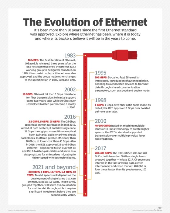
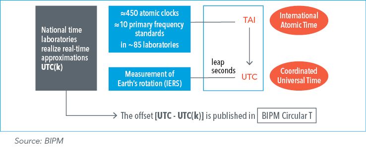