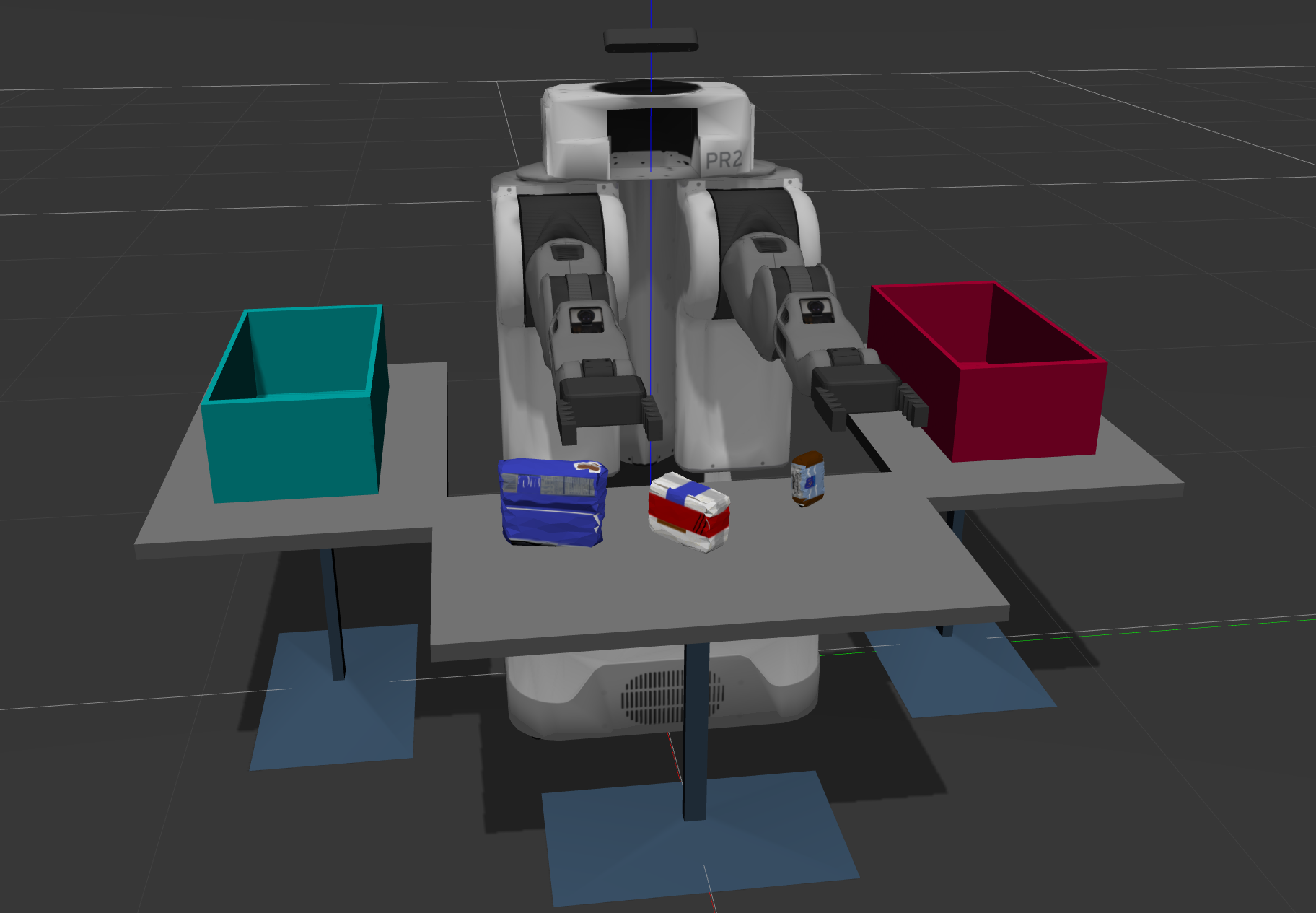
using pr2 robot which has RGB-D camera to perceive it's surrounding to pick specific object by defining it and place it in another specific place depending on the object itself, by performing analysis on the received data which has noise and distortion, by applying the filtering and segmentation techniques then object recognition and pose estimation to be able to tell the robot the position and orientation for each object.
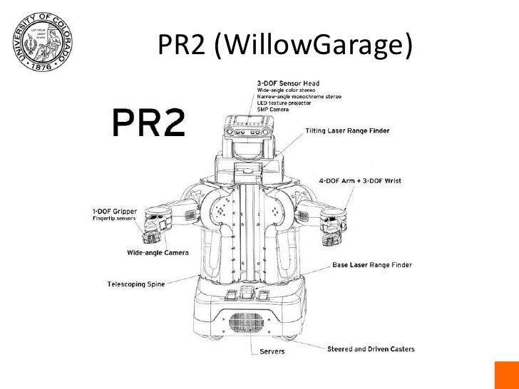
The PR2 is one of the most advanced research robots ever built. Its powerful hardware and software systems let it do things like clean up tables, fold towels, and fetch you drinks from the fridge.


- Imports
- helper functions
- pcl_callback() function
- Statistical Outlier Filtering
- Voxel Grid Downsampling
- PassThrough Filter
- RANSAC Plane Segmentation
- Euclidean Clustering
- Color Histograms
- normal Histograms
- object recognition
- PR2_Mover function
- Creating ROS Node, Subscribers, and Publishers
- environment setup and running
- Notes
using multiple python libraries like numpy sklearn pickle pickle and some ROS libraries
import numpy as np
import sklearn
from sklearn.preprocessing import LabelEncoder
import pickle
from sensor_stick.srv import GetNormals
from sensor_stick.features import compute_color_histograms
from sensor_stick.features import compute_normal_histograms
from visualization_msgs.msg import Marker
from sensor_stick.marker_tools import *
from sensor_stick.msg import DetectedObjectsArray
from sensor_stick.msg import DetectedObject
from sensor_stick.pcl_helper import *

import rospy
import tf
from geometry_msgs.msg import Pose
from std_msgs.msg import Float64
from std_msgs.msg import Int32
from std_msgs.msg import String
from pr2_robot.srv import *
from rospy_message_converter import message_converter
import yamlusing some functions like get_normals make_yaml_dict send_to_yaml
# Helper function to get surface normals
def get_normals(cloud):
    get_normals_prox = rospy.ServiceProxy('/feature_extractor/get_normals', GetNormals)
    return get_normals_prox(cloud).cluster
# Helper function to create a yaml friendly dictionary from ROS messages
def make_yaml_dict(test_scene_num, arm_name, object_name, pick_pose, place_pose):
yaml_dict = {}
yaml_dict["test_scene_num"] = test_scene_num.data
yaml_dict["arm_name"] = arm_name.data
yaml_dict["object_name"] = object_name.data
yaml_dict["pick_pose"] = message_converter.convert_ros_message_to_dictionary(pick_pose)
yaml_dict["place_pose"] = message_converter.convert_ros_message_to_dictionary(place_pose)
#print ("third")
return yaml_dict# Helper function to output to yaml file
def send_to_yaml(yaml_filename, dict_list):
data_dict = {"object_list": dict_list}
with open(yaml_filename, 'w') as outfile:
yaml.dump(data_dict, outfile, default_flow_style=False)
print ("done!")this function include filtering, segmentation and object recognition parts
it will be called back every time a message is published to /pr2/world/points
def pcl_callback(pcl_msg):

    ##########################################
    # first part :- filtering and segmentation
    ##########################################


    # first by converting the ros message type to pcl data
    cloud_filtered = ros_to_pcl(pcl_msg)

While calibration takes care of distortion, noise due to external factors like dust in the environment, humidity in the air, or presence of various light sources lead to sparse outliers which corrupt the results even more.
Such outliers lead to complications in the estimation of point cloud characteristics like curvature, gradients, etc. leading to erroneous values, which in turn might cause failures at various stages in our perception pipeline.
One of the filtering techniques used to remove such outliers is to perform a statistical analysis in the neighborhood of each point, and remove those points which do not meet a certain criteria. PCL’s StatisticalOutlierRemoval filter is an example of one such filtering technique. For each point in the point cloud, it computes the distance to all of its neighbors, and then calculates a mean distance.
    # due to external factors like dust in the environment we apply Outlier Removal Filter
    # taking the number of neighboring points = 4 & threshold scale factor = .00001
    outlier_filter = cloud_filtered.make_statistical_outlier_filter()
    outlier_filter.set_mean_k(4)
    x = 0.00001
    outlier_filter.set_std_dev_mul_thresh(x)
    cloud_filtered = outlier_filter.filter()
 big difference !!
RGB-D cameras provide feature rich and particularly dense point clouds, meaning, more points are packed in per unit volume than, for example, a Lidar point cloud. Running computation on a full resolution point cloud can be slow and may not yield any improvement on results obtained using a more sparsely sampled point cloud.
So, in many cases, it is advantageous to downsample the data. In particular, you are going to use a VoxelGrid Downsampling Filter to derive a point cloud that has fewer points but should still do a good job of representing the input point cloud as a whole.
    # using VoxelGrid Downsampling Filter to derive a point cloud that has fewer points
    # Creating a VoxelGrid filter object taking the leaf-size = .01
    vox = cloud_filtered.make_voxel_grid_filter()
    LEAF_SIZE = 0.01
    vox.set_leaf_size(LEAF_SIZE, LEAF_SIZE, LEAF_SIZE)
cloud_filtered = vox.filter() done! : low points per unit volume
The Pass Through Filter works much like a cropping tool, which allows you to crop any given 3D point cloud by specifying an axis with cut-off values along that axis. The region you allow to pass through, is often referred to as region of interest.
Applying a Pass Through filter along z axis (the height with respect to the ground) to our tabletop scene in the range 0.61 to 1.1
    passthrough = cloud_filtered.make_passthrough_filter()
    filter_axis = 'z'
    passthrough.set_filter_field_name(filter_axis)
    axis_min = 0.61
    axis_max = 1.1
    passthrough.set_filter_limits(axis_min, axis_max)
    cloud_filtered = passthrough.filter()
Applying a Pass Through filter along y axis (for horizontal axis) to our tabletop scene in the range -0.45 to 0.45
    passthrough = cloud_filtered.make_passthrough_filter()
    filter_axis = 'y'
    passthrough.set_filter_field_name(filter_axis)
    axis_min = -0.45
    axis_max = 0.45
    passthrough.set_filter_limits(axis_min, axis_max)
cloud_filtered = passthrough.filter() done! : the region has been specified
to remove the table itself from the scene. a popular technique known as Random Sample Consensus or "RANSAC". RANSAC is an algorithm, that can be used to identify points in the dataset that belong to a particular model.
The RANSAC algorithm assumes that all of the data in a dataset is composed of both inliers and outliers, where inliers can be defined by a particular model with a specific set of parameters, while outliers do not fit that model and hence can be discarded. Like in the example below, we can extract the outliners that are not good fits for the model.
If there is a prior knowledge of a certain shape being present in a given data set, we can use RANSAC to estimate what pieces of the point cloud set belong to that shape by assuming a particular model.
    # using The RANSAC algorithm to remove the table from the scene
    # by Creating the segmentation object and Setting the model
    # setting the max_distance then extracting the inliers and outliers
    seg = cloud_filtered.make_segmenter()
    seg.set_model_type(pcl.SACMODEL_PLANE)
    seg.set_method_type(pcl.SAC_RANSAC)
    max_distance =0.01
    seg.set_distance_threshold(max_distance)
    inliers, coefficients = seg.segment()

    # Extract inliers and outliers
    extracted_table = cloud_filtered.extract(inliers, negative=False)
    extracted_objects = cloud_filtered.extract(inliers, negative=True)
 done! : object and table have been extracted
DBSCAN stands for Density-Based Spatial Clustering of Applications with Noise.
The DBSCAN algorithm creates clusters by grouping data points that are within some threshold distance from the nearest other point in the data.
The DBSCAN Algorithm is sometimes also called “Euclidean Clustering”, because the decision of whether to place a point in a particular cluster is based upon the “Euclidean distance” between that point and other cluster members.
    # using a PCL library to perform a DBSCAN cluster search
    # first convert XYZRGB to XYZ then Create a cluster extraction object
    # then by Settin the tolerances for distance threshold, minimum and maximum cluster size
    # then Search the k-d tree for clusters and Extract indices for each of the discovered clusters
    white_cloud = XYZRGB_to_XYZ(extracted_objects)
    tree = white_cloud.make_kdtree()
    ec = white_cloud.make_EuclideanClusterExtraction()
    ec.set_ClusterTolerance(0.015)
    ec.set_MinClusterSize(1)
    ec.set_MaxClusterSize(50000)
    ec.set_SearchMethod(tree)
    cluster_indices = ec.Extract()
visualize the results in RViz! by creating another point cloud of type PointCloud_PointXYZRGB.
    # final step is to visualize the results in RViz!
    # by creating another point cloud of type PointCloud_PointXYZRGB
    cluster_color = get_color_list(len(cluster_indices))
    color_cluster_point_list = []
    for j, indices in enumerate(cluster_indices):
        for i, indice in enumerate(indices):
            color_cluster_point_list.append([white_cloud[indice][0],
                                            white_cloud[indice][1],
                                            white_cloud[indice][2],
                                             rgb_to_float(cluster_color[j])])
    cluster_cloud = pcl.PointCloud_PointXYZRGB()
    cluster_cloud.from_list(color_cluster_point_list)


    ros_cluster_cloud = pcl_to_ros(cluster_cloud)
    ros_cloud_objects = pcl_to_ros(extracted_objects)
ros_cloud_table = pcl_to_ros(extracted_table) pcl_objects_pub.publish(ros_cloud_objects)
pcl_table_pub.publish(ros_cloud_table)
pcl_cluster_pub.publish(ros_cluster_cloud)a color histogram is a representation of the distribution of colors in an image. For digital images, a color histogram represents the number of pixels that have colors in each of a fixed list of color ranges, that span the image's color space, the set of all possible colors.
def compute_color_histograms(cloud, using_hsv=False):

    # Compute histograms for the clusters
    point_colors_list = []

    # Step through each point in the point cloud
    for point in pc2.read_points(cloud, skip_nans=True):
        rgb_list = float_to_rgb(point[3])
        if using_hsv:
            point_colors_list.append(rgb_to_hsv(rgb_list) * 255)
        else:
            point_colors_list.append(rgb_list)

    # Populate lists with color values
    channel_1_vals = []
    channel_2_vals = []
    channel_3_vals = []

    for color in point_colors_list:
        channel_1_vals.append(color[0])
        channel_2_vals.append(color[1])
        channel_3_vals.append(color[2])

    L1_hist = np.histogram(channel_1_vals, bins=32, range=(0, 256))
    L2_hist = np.histogram(channel_2_vals, bins=32, range=(0, 256))
    L3_hist = np.histogram(channel_3_vals, bins=32, range=(0, 256))

    hist_features = np.concatenate((L1_hist[0], L2_hist[0], L3_hist[0])).astype(np.float64)
    norm_features = hist_features / np.sum(hist_features)

    return norm_features
a normal histogram is a representation of the distribution of normals to the shape in an image
def compute_normal_histograms(normal_cloud):
    norm_x_vals = []
    norm_y_vals = []
    norm_z_vals = []

    for norm_component in pc2.read_points(normal_cloud,
                                          field_names = ('normal_x', 'normal_y', 'normal_z'),
                                          skip_nans=True):
        norm_x_vals.append(norm_component[0])
        norm_y_vals.append(norm_component[1])
        norm_z_vals.append(norm_component[2])

    # TODO: Compute histograms of normal values (just like with color)
    S1_hist = np.histogram(norm_z_vals, bins=32, range=(0, 256))
    S2_hist = np.histogram(norm_z_vals, bins=32, range=(0, 256))
    S3_hist = np.histogram(norm_z_vals, bins=32, range=(0, 256))

    hist_features = np.concatenate((S1_hist[0], S2_hist[0], S3_hist[0])).astype(np.float64)
    normed_features = hist_features / np.sum(hist_features)

    return normed_features
Support Vector Machine or "SVM" is just a funny name for a particular supervised machine learning algorithm that allows you to characterize the parameter space of your dataset into discrete classes.
SVMs work by applying an iterative method to a training dataset, where each item in the training set is characterized by a feature vector and a label.
    #########################################
    # second part :- object recognition
    #########################################


    # Classify the clusters
    detected_objects_labels = []
    detected_objects = []

    # loop to cycle through each of the segmented clusters
    for index, pts_list in enumerate(cluster_indices):

        # Grab the points for the cluster
        pcl_cluster = extracted_objects.extract(pts_list)

        # convert the cluster from pcl to ROS
        ros_cluster = pcl_to_ros(pcl_cluster)

        # Extract histogram features
        color_hists = compute_color_histograms(ros_cluster, using_hsv=True)
        normals = get_normals(ros_cluster)
        normal_hists = compute_normal_histograms(normals)
        feature = np.concatenate((color_hists, normal_hists))

        # Make the prediction, retrieve the label for the result
        # and add it to detected_objects_labels list
        prediction = clf.predict(scaler.transform(feature.reshape(1,-1)))
        label = encoder.inverse_transform(prediction)[0]
        detected_objects_labels.append(label)

        # Publish a label into RViz
        label_pos = list(white_cloud[pts_list[0]])
        label_pos[2] += .2
        object_markers_pub.publish(make_label(label,label_pos, index))

        # Add the detected object to the list of detected objects.
        do = DetectedObject()
        do.label = label
        do.cloud = ros_cluster
        detected_objects.append(do)

    rospy.loginfo('Detected {} objects: {}'.format(len(detected_objects_labels), detected_objects_labels))

    # Publish the list of detected objects
    detected_objects_pub.publish(detected_objects)

    # Suggested location for where to invoke your pr2_mover() function within pcl_callback()
    # Could add some logic to determine whether or not your object detections are robust
    # before calling pr2_mover()
    try:
        pr2_mover(detected_objects)

    except rospy.ROSInterruptException:
        pass


    object_name = String()
    test_scene_num = Int32()
    pick_pose = Pose()
    place_pose = Pose()
arm_name = String() # Get/Read parameters
object_list_param = rospy.get_param('/object_list')
dropbox_param = rospy.get_param('/dropbox')
test_scene_num.data = 2
yaml_dict_list = []
labels = []
centroids = []
# access the (x, y, z) coordinates of each point and compute the centroid
for object in object_list:
labels.append(object.label)
points_arr = ros_to_pcl(object.cloud).to_array()
centroids.append(np.mean(points_arr, axis=0)[:3])then we have to loop through the pick list to calc the pick pose and the place pose then we have to Create a list of dictionaries for yaml.
    for i in range(0, len(object_list_param)):
        # get the object name and group from object list
        object_name.data = object_list_param[i]['name']
        object_group = object_list_param[i]['group']

        try:
            index = labels.index(object_name.data)
        except ValueError:
            print "Object not detected: %s" %object_name.data
            continue

        # get the pick pose and place pose
        pick_pose.position.x = np.asscalar(centroids[index][0])
        pick_pose.position.y = np.asscalar(centroids[index][1])
        pick_pose.position.z = np.asscalar(centroids[index][2])

        selected_dic = [element for element in dropbox_param if element['group'] == object_group][0]
        position = selected_dic.get('position')
        place_pose.position.x = position[0]
        place_pose.position.y = position[1]
        place_pose.position.z = position[2]

        # to know wich arm to be used
        selected_dic = [element for element in dropbox_param if element['group'] == object_group][0]
        arm_name.data = selected_dic.get('name')

        # Create a list of dictionaries for yaml
        yaml_dict = make_yaml_dict(test_scene_num, arm_name, object_name, pick_pose, place_pose)
        yaml_dict_list.append(yaml_dict)

        # Wait for 'pick_place_routine' service to come up
        rospy.wait_for_service('pick_place_routine')
        try:
            pick_place_routine = rospy.ServiceProxy('pick_place_routine', PickPlace)
            resp = pick_place_routine(test_scene_num, object_name, arm_name, pick_pose, place_pose)
            print ("Response: ",resp.success)
        except rospy.ServiceException, e:
print "Service call failed: %s"%e # get the output in yaml format
yaml_filename = 'output_'+str(test_scene_num.data)+'.yaml'
send_to_yaml(yaml_filename, yaml_dict_list)if __name__ == '__main__':
# ROS node initialization
rospy.init_node('clustering', anonymous=True) # Create Subscribers
pcl_sub = rospy.Subscriber("/pr2/world/points", pc2.PointCloud2, pcl_callback, queue_size=1)
# Create Publishers
pcl_objects_pub = rospy.Publisher("/pcl_objects", PointCloud2, queue_size=1)
pcl_table_pub = rospy.Publisher("/pcl_table", PointCloud2, queue_size=1)
pcl_cluster_pub = rospy.Publisher("/pcl_cluster", PointCloud2, queue_size=1)
object_markers_pub = rospy.Publisher("/object_markers", Marker, queue_size=1)
detected_objects_pub = rospy.Publisher("/detected_objects", DetectedObjectsArray, queue_size=1)now we cat load the model data from the disc, and as the node is still active we will spin our code.
    # Load Model From disk
    model = pickle.load(open('model.sav', 'rb'))
    clf = model['classifier']
    encoder = LabelEncoder()
    encoder.classes_ = model['classes']
    scaler = model['scaler']

    # Initialize color_list
    get_color_list.color_list = []

    # Spin while node is not shutdown
    while not rospy.is_shutdown():
rospy.spin()For this setup, catkin_ws is the name of active ROS Workspace, if your workspace name is different, change the commands accordingly If you do not have an active ROS workspace, you can create one by:
$ mkdir -p ~/catkin_ws/src
$ cd ~/catkin_ws/
$ catkin_make
Now that you have a workspace, clone or download this repo into the src directory of your workspace:
$ cd ~/catkin_ws/src
$ git clone https://github.com/mohamedsayedantar/RoboND-Perception-Project.get
Note: If you have the Kinematics Pick and Place project in the same ROS Workspace as this project, please remove the 'gazebo_grasp_plugin' directory from the RoboND-Perception-Project/ directory otherwise ignore this note.
Now install missing dependencies using rosdep install:
$ cd ~/catkin_ws
$ rosdep install --from-paths src --ignore-src --rosdistro=kinetic -y
Build the project:
$ cd ~/catkin_ws
$ catkin_make
Add following to your .bashrc file
export GAZEBO_MODEL_PATH=~/catkin_ws/src/RoboND-Perception-Project/pr2_robot/models:$GAZEBO_MODEL_PATH
If you haven’t already, following line can be added to your .bashrc to auto-source all new terminals
source ~/catkin_ws/devel/setup.bash
To run the project:
$ roslaunch pr2_robot pick_place_project.launchand in another terminal:
$ cd ~/catkin_ws/src/RoboND-Perception-Project/pr2_robot/scripts
$ chmod u+x project_template.py
$ cd ~/catkin_ws
$ rosrun pr2_robot project_template.pyyou can change the objects in capture_features.py file in sensor_stick/scripts with the objects for each world.
these objects can be found in pick_list_*.yaml files in /pr2_robot/config/ now we can Generate the Features:
$ cd ~/catkin_ws
$ roslaunch sensor_stick training.launch$ rosrun sensor_stick capture_features.py$ rosrun sensor_stick train_svm.pyto change the world itself in Gazebo and RViz we can change pick_list_1 and test1 in pick_place_project.launch file in the /pr2_robot/config directory to choose any world from the 3 worlds
    <!--TODO:Change the world name to load different tabletop setup-->
    <arg name="world_name" value="$(find pr2_robot)/worlds/test1.world"/>
    <!--TODO:Change the list name based on the scene you have loaded-->
    <rosparam command="load" file="$(find pr2_robot)/config/pick_list_1.yaml"/>
the normalized confusion matrices and the confusion matrices without normalization --> for the 3 worlds


in the world 3 after running rosrun pr2_robot project_template.py this error will occur:

to solve this error go to features.py file in sensor_stick/src/sensor_stick to modify the np.histogram method in compute_normal_histograms function by changing the range from range=(0, 256) to range=(-1, 1) to solve this error.
the 3 worlds model.sav files is existed in the RoboND-Perception-Project directory as model_*.sav