Ray tracing is a rendering technique widely used in computer graphics. In short, the principle of ray tracing is to trace the path of the light through each pixel, and simulate how the light beam encounters an object. Unlike rasterization technique which focuses on the realistic geometry of objects, ray tracing focuses on the simulation of light transport, where each ray is computational independent. This feature makes ray tracing suitable for a basic level of parallelization.
Due to the characteristics of ray tracing algorithms, it is straightforward to convert the serial code into a parallel one, and the given code already implements a CPU-based parallel approach using OpenMP, where each image row runs in parallel. For the GPU parallel approach, we can use two-dimensional thread blocks and grids, in which each thread does computation for one pixel or a block of subpixels.
However, because of the divergence of ray paths, the computational workload of each pixel is different. Thus it is hard to achieve high utilization and low overhead under parallelization. Therefore, computation uniformity and work balance should be taken care of to optimize the performance.
Currently there are many available codes to generate images using ray tracing algorithms, which can run on CPU or GPU in single or multi-thread methods. Existing CPU-based parallel approaches include dynamic scheduling and shared memory multiprocessing using OpenMP.
For GPU-based parallelism, there are various papers on this topic that target specific algorithms or data structures that can be used in ray tracing and implement new optimized structures suitable for GPU computing. In 2018, the announcements of NVIDIA’s new Turing GPUs, RTX technology spurred a renewed interest in ray tracing. NVIDIA gave a thorough walk through of translating C++ code to CUDA that results in a 10x or more speed improvement in their book Ray Tracing in One Weekend.
Our parallel strategy for ray tracing is quite straightforward: just let each thread do computation for one pixel. First, we to read the scene to be rendered. The spheres are then saved in a host array. Memory for spheres and the output image is allocated on the device and copied from the host.
Second, we set the grid dimension and block dimension, using 2-dimensional thread blocks to cover the whole image, where each thread does its own calculation for one pixel. Then kernel render() is executed where ray tracing of multiple samples in one pixel is conducted.
The processing of the image has been done in square batches of pixels (e.g., 8 by 8 batch). Four kernels are called, the first two of which are used for initializing and setting up the type of scene that needs to be rendered and the next two kernels have been used to initialize the random numbers for each thread while rendering the required image respectively. In the serial implementation, we have used nested for loops to iterate over all of the pixels. In CUDA, the scheduler takes blocks of threads and schedules them on the GPU for us. CUDA allows us to maintain a Unified Memory frame buffer that is written by the GPU and read by the CPU. The serial implementation to compute the color of a surface when translated to CUDA code results in a stack overflow since it can call itself many times. So, it had to be changed to iteratively compute the color of the desired pixel. The number of iterations can be varied as the max recursive depth of the serial implementation.
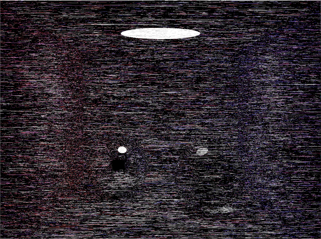
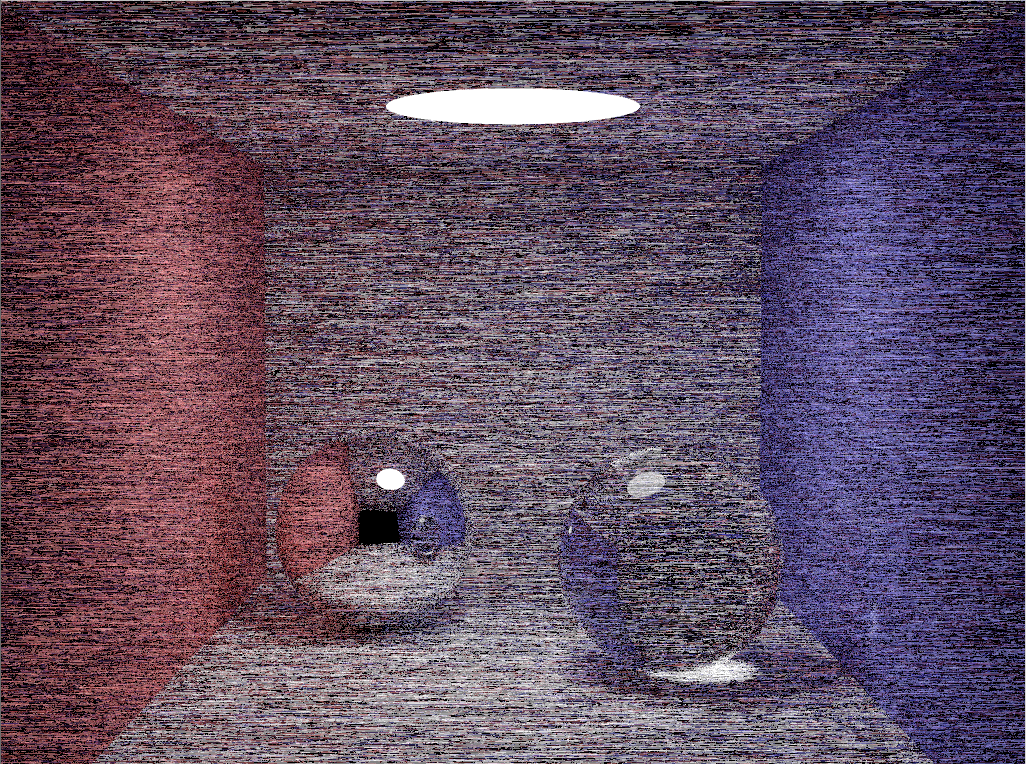
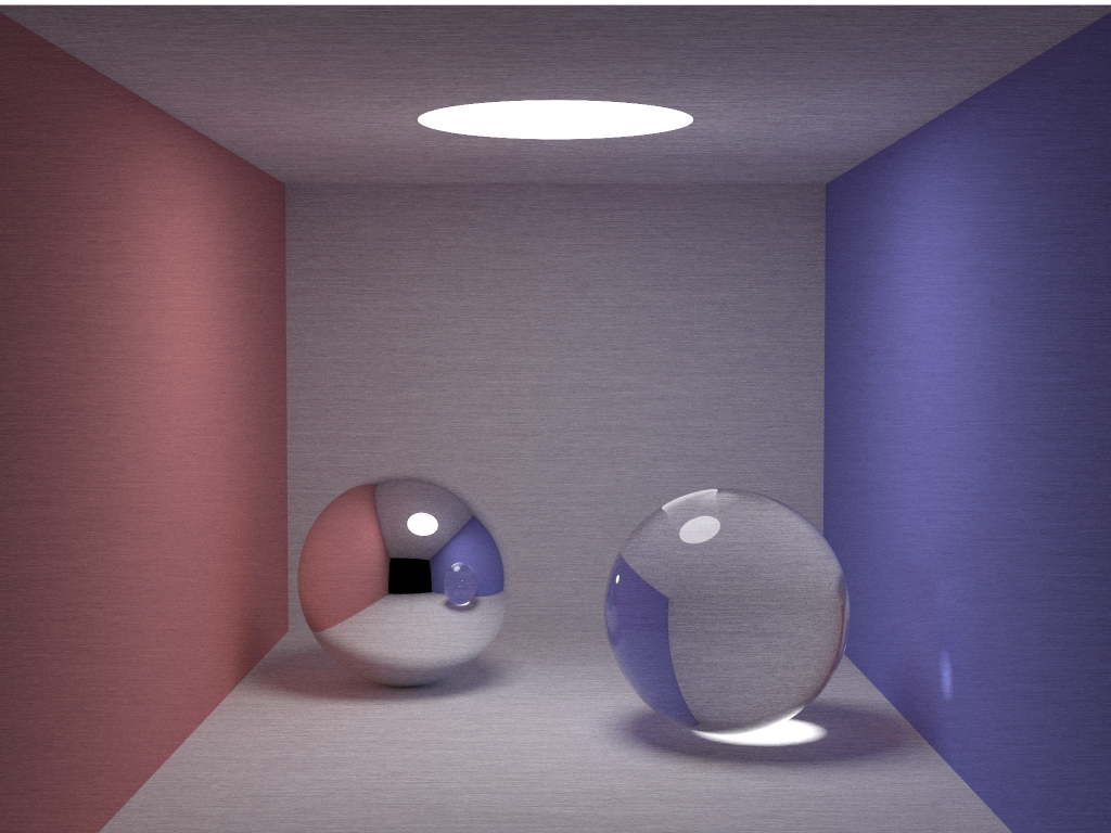
The following images were obtained with different samples per pixel.
 |
 |
|---|---|
| spp = 8 | spp = 40 |
 |
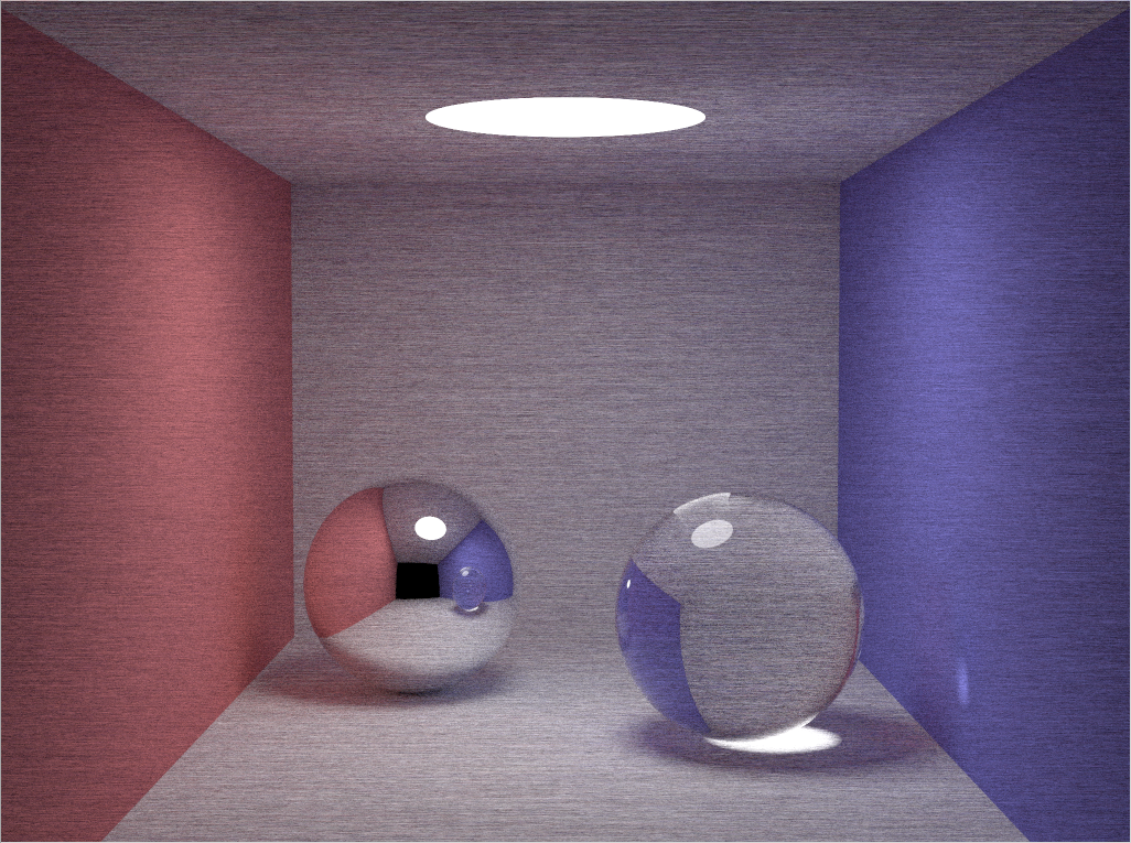 |
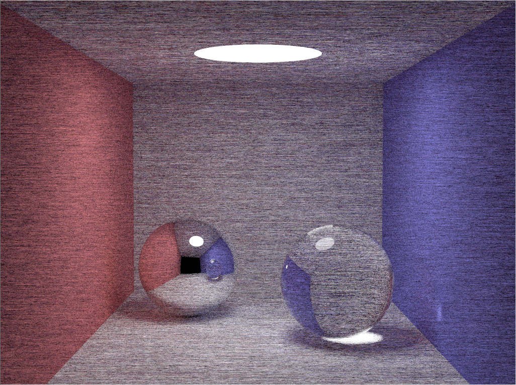
| spp = 200 | spp = 1000 |
 |
 |
| spp = 2000 | spp = 5000 |
Here we compare our CUDA parallel version with the given CPU code using OpenMP parallelization.
| Time (s) | ||||||
|---|---|---|---|---|---|---|
| spp | 8 | 40 | 200 | 1000 | 2000 | 5000 |
| CPU | 0.99 | 4.24 | 20.00 | 98.58 | 201.15 | 510.22 |
| GPU | 0.68 | 0.83 | 1.30 | 3.50 | 6.32 | 14.63 |
| Speedup | 1.46 | 5.11 | 15.38 | 28.17 | 31.83 | 34.87 |
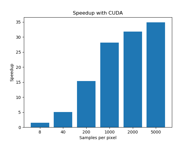
As we can see, GPU parallelization with CUDA achieves a great speedup in execution time, which initially proved the correctness of our parallelization approach.
GPU Speed of Light
| Baseline | With Optimization 1,2&3 | Improvement (%) | |
|---|---|---|---|
| Time (s) | 3.03 | 2.48 | -18.15% |
| SoL SM (%) | 38.48 | 67.66 | +75.84% |
| SoL Memory (%) | 67.18 | 15.57 | -76.82% |
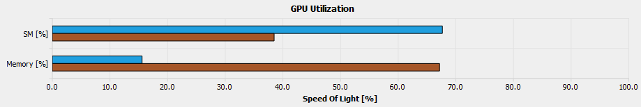
In all, we successfully optimized the usage of SM by 75.84%, and reduced the memory throughput by 76.82%. The improvement of time was not very significant compared with other factors, but it achieved a lower baseline.
Memory Workload
| Baseline | With Optimization 1,2&3 | Improvement (%) | |
|---|---|---|---|
| Memory Throughput (GB/s) | 437.63 | 0.211 | -99.95% |
| Global Load Cached | 11.57G | 19.88G | +71.80% |
| Local Load Cached | 4.89G | 0 | -100% |
| Shared Load | 0 | 0 | 0 |
| Global Store | 294K | 294K | 0 |
| Local Store | 4.09G | 0.77G | -81.23% |
| L1 Hit Rate (%) | 64.13 | 99.99 | +55.91% |
By converting 4.98G local load into global load, we could successfully obtain a L1 cache hit of 99.99% , thus decreasing memory throughput by 99.95% without using shared memory.
Scheduler Statistics
| Baseline | With Optimization 1,2&3 | Improvement (%) | |
|---|---|---|---|
| Theoretical Warps / Scheduler | 16 | 16 | 0 |
| Active Warps / Scheduler | 3.91 | 3.92 | +0.18% |
| Eligible Warps / Scheduler | 0.29 | 0.73 | +149.88% |
| Issued Warps / Scheduler | 0.22 | 0.43 | +93.31% |
The improvement on eligible warps was significant by around 150%. There’s no obvious shift in active warps, and load balancing was still not optimal. It could be a limitation of the current parallel approach, since in the ray-tracing algorithm, the workload of each pixel (number of radiances) depends on the rendered scene itself.
Execution Time
Here we compare our optimized CUDA parallel code with the given CPU code using OpenMP parallelization. As we can see, the optimized version has a better speedup with an average improvement close to 18%. A speedup of more than 35x is achieved with a large data set.
| Time (s) | ||||||
|---|---|---|---|---|---|---|
| spp | 8 | 40 | 200 | 1000 | 2000 | 5000 |
| CPU | 0.99 | 4.24 | 20.00 | 98.58 | 201.15 | 510.22 |
| GPU | 0.68 | 0.83 | 1.30 | 3.50 | 6.32 | 14.63 |
| GPU w.o. | 0.57 | 0.70 | 1.07 | 2.95 | 5.36 | 13.60 |
| Speedup | 1.74 | 6.06 | 18.69 | 33.42 | 37.53 | 37.52 |

Accuracy
Here we plot the mean squared error vs. the execution time. As we can see, with samples per pixel more than 1000 can the target image achieve a target MSE of 52. 1000 spp is pretty close to the criteria, so let’s say using 1100 samples per pixel is safe enough to pass the threshold with an execution time under 5 seconds.
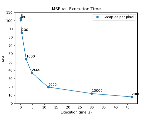
With 1100 samples per pixel, we obtained the final result with a MSE of 51.28 and an execution time of 3.09s.
From the speedup result of using CUDA for GPU parallelization, we realized the advantages of GPU over CPU in dense floating point arithmetic, for example image processing and matrix calculations. The architecture features of GPU makes it the best candidate for ray tracing acceleration.
Different from optimizations such as matrix multiplication, it could happen that some universal approval methods may not be useful under different scenarios. For example, using shared memory would not make a great difference in our project because memory bandwidth is not the bottleneck of performance. However, all of us finally admit that optimization is highly dependent on our algorithms as well.