AFM Bacteria Identification

Disclaimer

This Software tries to communicate directly with the neaSNOM Microscope using SDKs provided by neaspec GmbH. Without them this Software will not work. Also the developer takes no responsibility for any damage caused while using this program, so use with caution and at own risk.

General

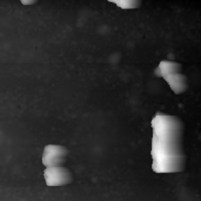
This project is build to work with a neaSNOM Microscope (neaspec GmbH, Germany), but should be easily expandable to work with other Device for Atomic Force Microscopy (AFM) as well. At the moment the Software uses the SDKs provided by neaspec to control the Microscope. It is based on the OpenCV Library and uses Canny Edge Detection as well as OpenCVs findContours() Function.

Basic Algorithm

Assuming you have two twodimensional Data Arrays representing two Measurement Directions that differ by 180° the Algorithms works like this (Code is in Python 3.6):

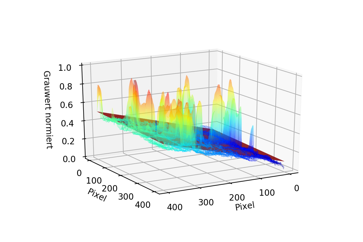
First both Arrays are leveld using linear regression. The function looks like this:

def plane_correction(raw):
    null_val = np.average(raw)
    raw[np.isnan(raw)] = null_val
    m = raw.shape
    X1, X2 = np.mgrid[:m[0], :m[1]]
    X = np.hstack((np.reshape(X1, (m[0]*m[1], 1)), np.reshape(X2, (m[0]*m[1], 1))))
    X = np.hstack((np.ones((m[0]*m[1], 1)), X))
    YY = np.reshape(raw, (m[0]*m[1], 1))
    theta = np.dot(np.dot(np.linalg.pinv(np.dot(X.transpose(), X)), X.transpose()), YY)
    plane = np.reshape(np.dot(X, theta), m)
    return (raw - plane)

After that the two directions are combined to 1 final data array.

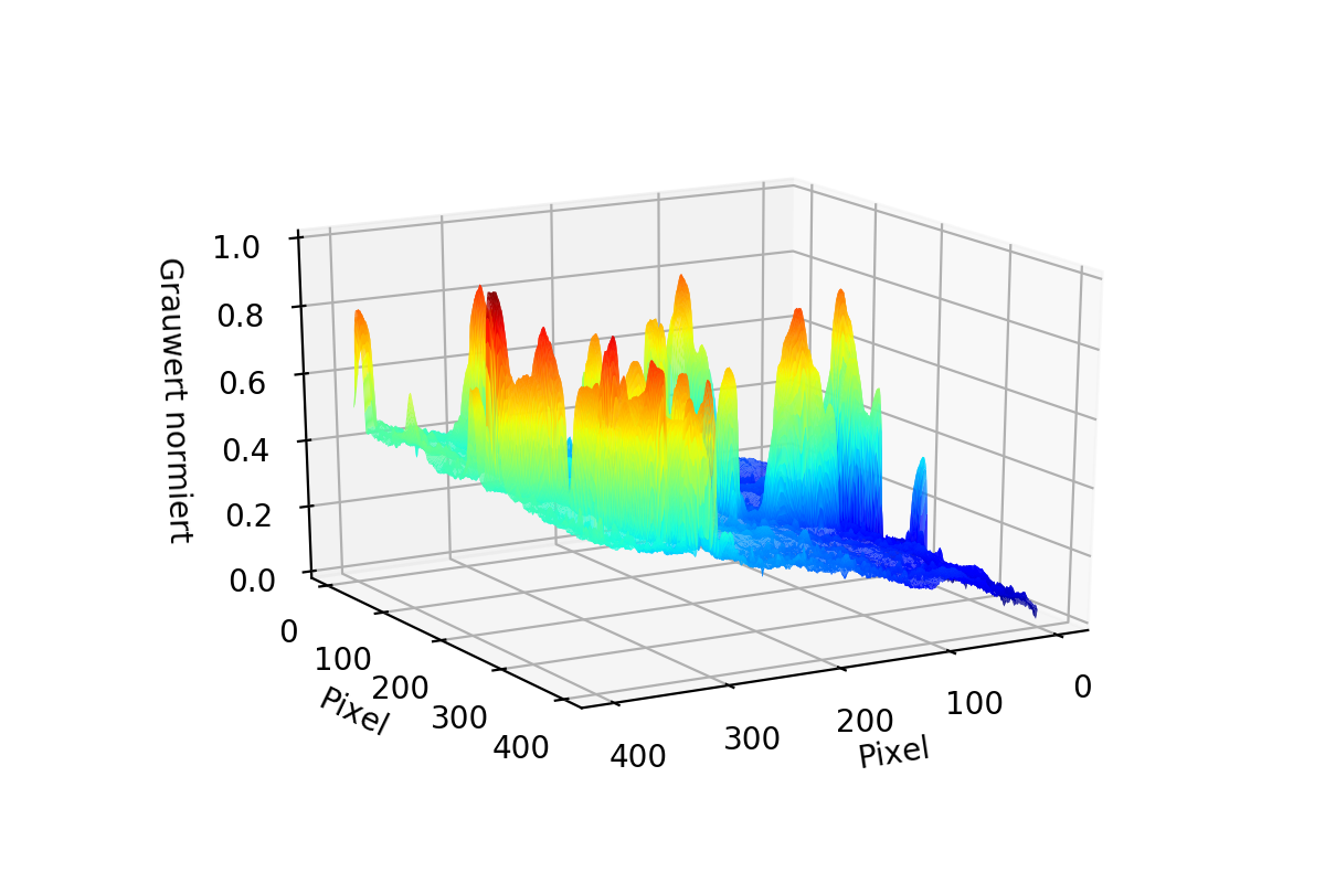
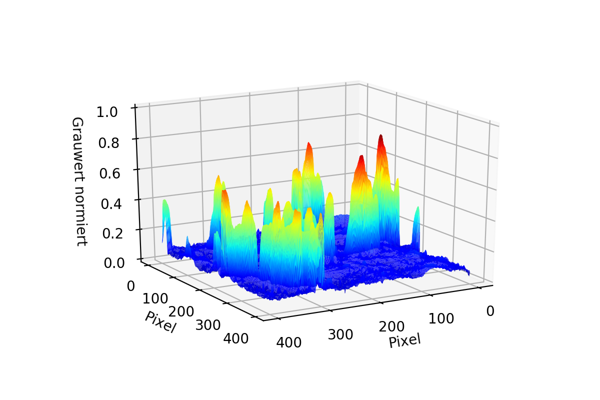
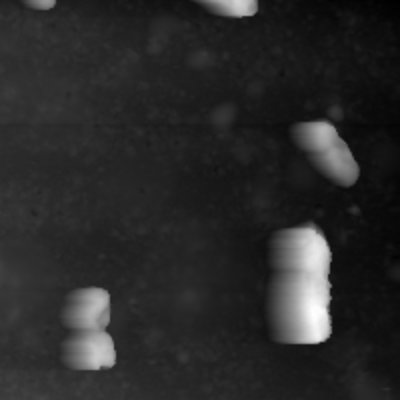
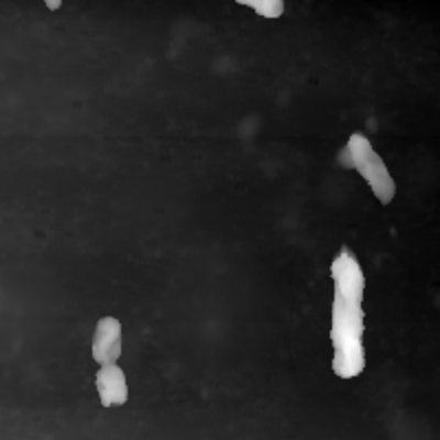
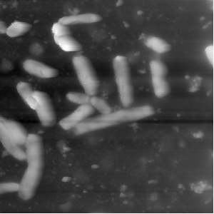
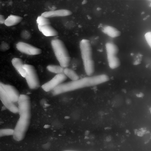
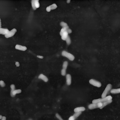
As you can see in the first two pictures it is possible for the data to have "Tails". To Correct them both Matrices are Stacked to 1D Arrays and then combined to one single Array using the smaller value of the two. The result is seen in the third image.

#z_data is left to right tip direction, r_data is right to left
comb_data = np.array([np.ndarray.flatten(z_data), np.ndarray.flatten(r_data)])
#self._shape saves the shape of the input Array
data = np.reshape(np.nanmin(comb_data, axis=0), self._shape)

After that possible stripes in the data are removed.

 for x in range(len(data)):
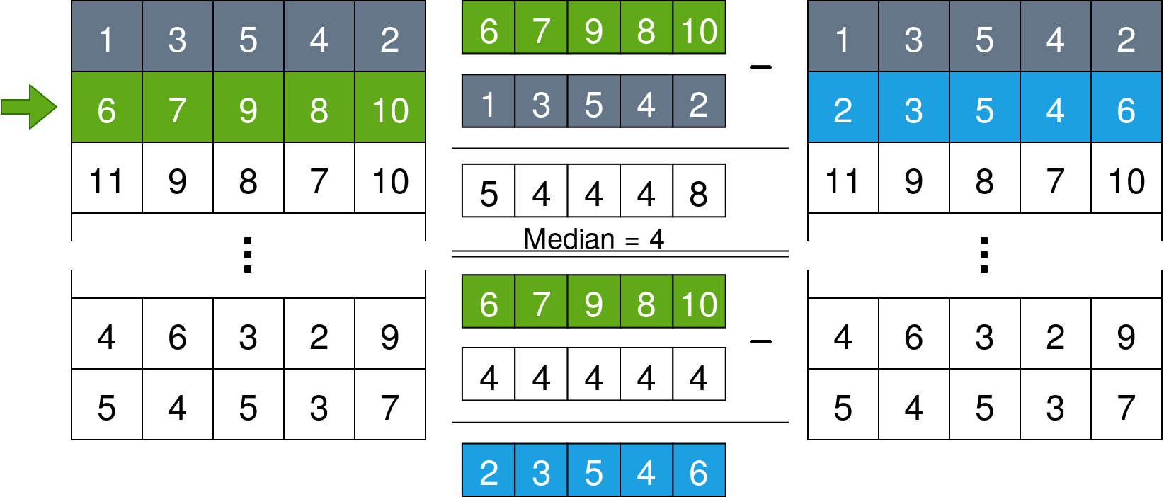
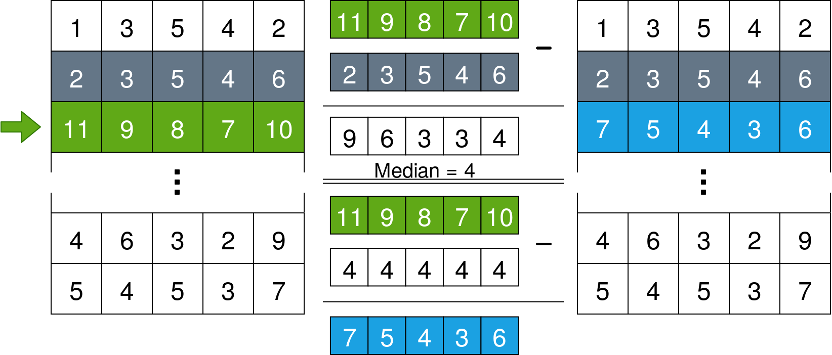
    data[x] = data[x] - np.median(data[x] - data[x-1])

What this does is iterate over the lines of the data array and set the median of the difference vector between each line and the line before it to 0. The following image explains it further:

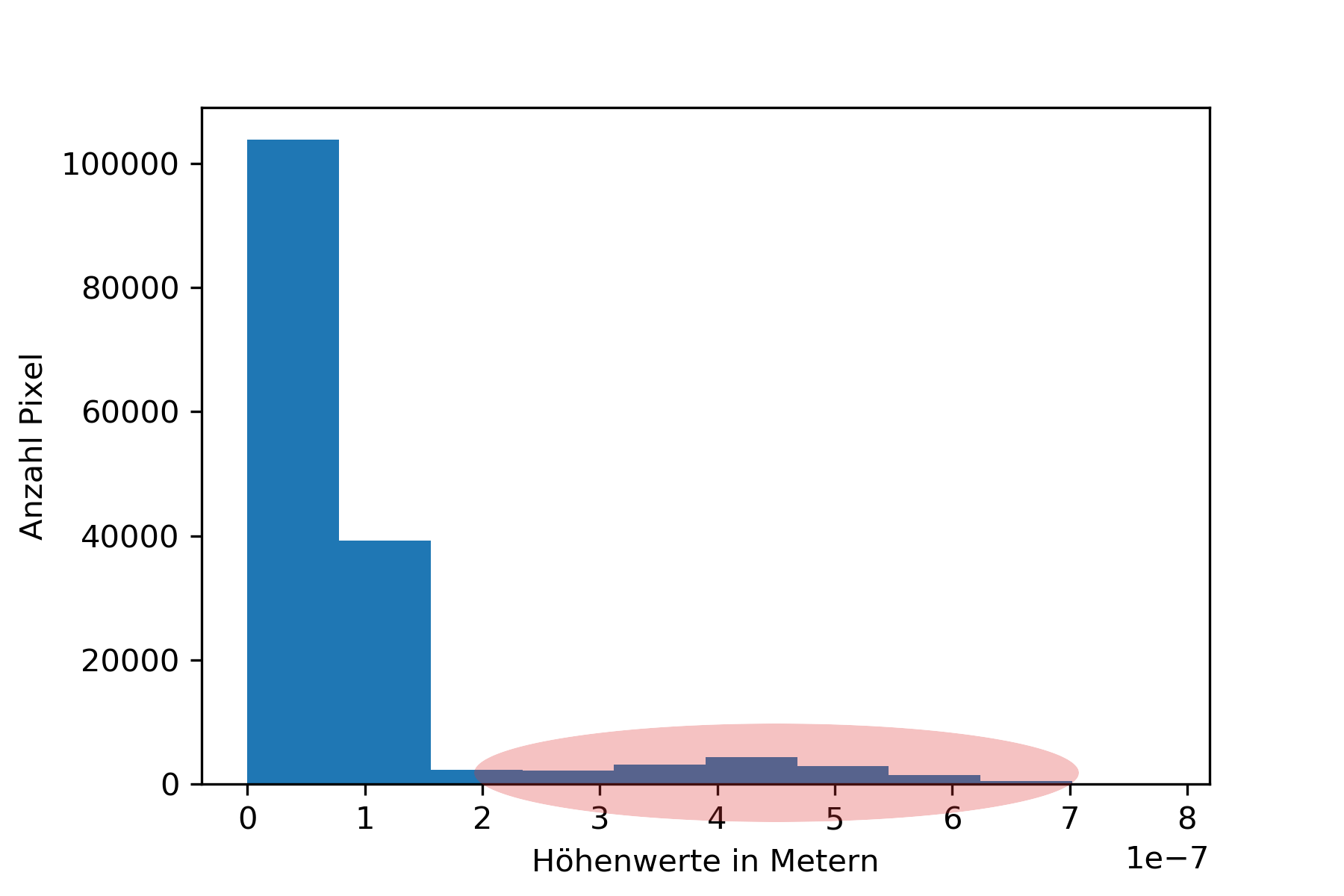
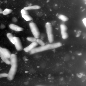
Next up the value range of the data is decreased by cutting off the top values. The next image shows an example of a histogram. The marked area shows the range in which the bacteria can be found. As you can see the values spread out a lot, so to increase the contrast between bacteria and background the values are cut off. The second and third image show a comparison for the bacteria image.

#limit is the value indicating where to cut off the data
data[np.where(data > limit)] = limit

The next steps are pretty common for edge detection. The data is normalized (left image) to greyscale values from 0 to 1 and a noise filter is applied (right image). The noise filter of choice is the bilateral filter