Update geoaxes.py pcolormesh overlapping cells plot issue #1416 #1418
Conversation
Commented out the part plotting the overlapping cells (despite a smaller zorder).
Now the overlapping cells larger than half the projection span stay masked.
lib/cartopy/mpl/geoaxes.py
Outdated
| # this method | ||
| collection._wrapped_collection_fix = pcolor_col | ||
|
|
||
| # the part below in comment retrieves the masked |
lib/cartopy/mpl/geoaxes.py
Outdated
| collection._wrapped_collection_fix = pcolor_col | ||
|
|
||
| # the part below in comment retrieves the masked | ||
| # overlapping cells and plot them with pcolor and a |
lib/cartopy/mpl/geoaxes.py
Outdated
| # the part below in comment retrieves the masked | ||
| # overlapping cells and plot them with pcolor and a | ||
| # smaller zorder to hide them | ||
| # but there are not always hidden |
lib/cartopy/mpl/geoaxes.py
Outdated
| # overlapping cells and plot them with pcolor and a | ||
| # smaller zorder to hide them | ||
| # but there are not always hidden | ||
| # if one wants to retrieve those cells, split them at the |
lib/cartopy/mpl/geoaxes.py
Outdated
| # smaller zorder to hide them | ||
| # but there are not always hidden | ||
| # if one wants to retrieve those cells, split them at the | ||
| # boundary and plot them, the code below could be |
lib/cartopy/mpl/geoaxes.py
Outdated
| # if one wants to retrieve those cells, split them at the | ||
| # boundary and plot them, the code below could be | ||
| # useful. | ||
|
|
There was a problem hiding this comment.
W293 blank line contains whitespace
lib/cartopy/mpl/geoaxes.py
Outdated
| # pcolor_data = np.ma.array(C, mask=~mask) | ||
| # | ||
| # pts = coords.reshape((Ny, Nx, 2)) | ||
| # |
fix trailing white spaces
|
We shouldn't be commenting out code, but just remove it if it's wrong. Before doing so, I'd really want to see some before and after comparisons, because that original code was added for a reason (that I haven't dug into yet to figure out). |
|
The part, I have commented out, plots with pcolor the overlapping cells that have been masked earlier. It plots them with a lower zorder. So if there was no land_mask or it the data were atmospheric data, they would not show. With oceanographic data, like ice concentration, those cells still appear on the plot despite their lower zorder. My understanding is that by keeping those cells, one can later process them to split them at the boundary and plot them correctly, that's why I kept the code commented out. Removing it would be cleaner and if one wants to process those cells, then one would have to change the code. |
 greglucas
left a comment
greglucas
left a comment
There was a problem hiding this comment.
It seems like this should be investigated a little more as to why the code was there in the first place.
Is the problem that these masked cells get passed through everything and then later on they get split into two cells (one on each side of the boundary) and only one of those cells keeps the mask, or it somehow changes the masking of the cell?
It seems like there is a more fundamental underlying problem here and that the masks should work in this situation and that would be worthwhile to look into. I'm thumbs down on this brute force comment out the block of code as it currently stands.
| # useful. | ||
|
|
||
| # ############# | ||
| # |
There was a problem hiding this comment.
What about making this a kwarg option, rather than commenting it out?
if kwargs['keep_bad_cells']:
    ...
| # if np.any(~pcolor_data.mask): | ||
| # # plot with slightly lower zorder to avoid odd issue | ||
| # # where the main plot is obscured | ||
| # zorder = collection.zorder - .1 |
There was a problem hiding this comment.
Did you try making this a much lower zorder like -1, so it is below all other artists?
There was a problem hiding this comment.
I tried a much lower order like -1.
In that case, it doesn't always work so I tried an ever larger number, and it worked.
Now I think there is no guarantee that it will always hid the cell, not plotting them is a better guarantee.
I think the issue comes with masked data, like oceanographic data with a land mask. I would say that when this was written, pushing the "hidden cell" behind the good one, was good enough, but when there is no data on the land mask, then the cells behind still appear on the masked area, not obscuring the data but the mask, and still making a mess of the plot.
Making it a kwargs is a possible option.
The idea was that those cell had to be hidden, so let's hide them efficiently. I admit that I spend quite some time thinking about it and I am sure of one thing is that cartopy needs to get rid of the cells...
|
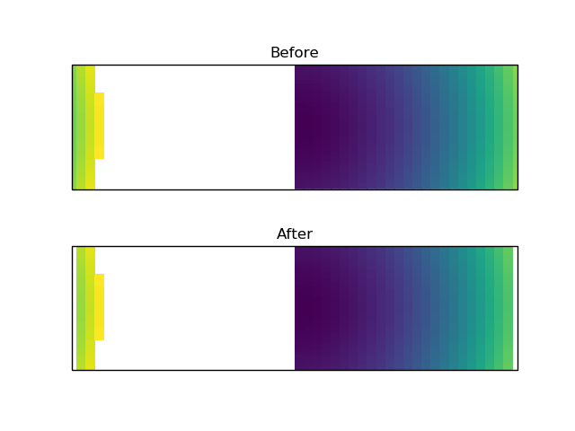
I just took a little closer look at this, and I think it is important to keep those lines in there for boundary wrapping purposes. For your cases could you use In general, though, I think those cells need to be replotted to appear on the boundaries as demonstrated below. import numpy as np
import matplotlib.pyplot as plt
import cartopy.crs as ccrs
fig, (ax1, ax2) = plt.subplots(nrows=2, subplot_kw={'projection': ccrs.Mercator()})
x = np.linspace(0, 360)
y = np.linspace(-45, 45)
X, Y = np.meshgrid(x, y)
Z = np.ma.masked_greater(X**2 + Y**2, 200**2)
mesh1 = ax1.pcolormesh(X, Y, Z, transform=ccrs.PlateCarree())
mesh2 = ax2.pcolormesh(X, Y, Z, transform=ccrs.PlateCarree())
mesh2._wrapped_collection_fix.set_visible(False)
ax1.set_title('Before')
ax2.set_title('After')
plt.show() |
|
Hi,
I am not sure what you mean.
Plotting the overlapping cells doesn’t improve the boundary, because they are plotted across the plot, not through the boundary.
On this example (which shows the overlapping cells on the bottoms plots), we can see that the boundaries are white, because the overlapping cells are plotted across the plot.
So I don’t see the what plotting those overlapping cells could bring.
Of course, if we want them to cross the plot, this is an other issue.
… Le 15 févr. 2020 à 22:45, Greg ***@***.***> a écrit :
I just took a little closer look at this, and I think it is important to keep those lines in there for boundary wrapping purposes. For your cases could you use mesh._wrapped_collection_fix.set_visible(False)?
In general, though, I think those cells need to be replotted to appear on the boundaries as demonstrated below.
<https://user-images.githubusercontent.com/12417828/74595658-88e32b80-5001-11ea-82a1-2a182d620f70.png>
import numpy as np
import matplotlib.pyplot as plt
import cartopy.crs as ccrs

fig, (ax1, ax2) = plt.subplots(nrows=2, subplot_kw={'projection': ccrs.Mercator()})

x = np.linspace(0, 360)
y = np.linspace(-45, 45)
X, Y = np.meshgrid(x, y)
Z = np.ma.masked_greater(X**2 + Y**2, 200**2)

mesh1 = ax1.pcolormesh(X, Y, Z, transform=ccrs.PlateCarree())
mesh2 = ax2.pcolormesh(X, Y, Z, transform=ccrs.PlateCarree())
mesh2._wrapped_collection_fix.set_visible(False)

ax1.set_title('Before')
ax2.set_title('After')

plt.show()
—
You are receiving this because you authored the thread.
Reply to this email directly, view it on GitHub <#1418?email_source=notifications&email_token=ANCCYW6W5QFATF5MLHLRW6TRDBO6VA5CNFSM4J2KPIN2YY3PNVWWK3TUL52HS4DFVREXG43VMVBW63LNMVXHJKTDN5WW2ZLOORPWSZGOEL3XWCI#issuecomment-586644233>, or unsubscribe <https://github.com/notifications/unsubscribe-auth/ANCCYW6I4PNTCAX26WDZJWTRDBO6VANCNFSM4J2KPINQ>.
|
|
I apologize, I wasn't very clear in the previous message. I think the "Before" in the image above is the correct way of doing things. In the second "After" image, the cells that cross the boundary are masked and removed from the plot (same as commenting out the lines of code). Note that I haven't looked into the full transformation path, but I think what is happening is:
That is why I think this code path is important to leave in, we want those two extra Polygons to go right up to the border on each side of the map, not to just ignore them. Perhaps this means that the boundary needs to be defined at a higher resolution for the actual clip paths being used? I'm not sure if #1422 will help here with the clipping or not. I think that your other PR #1420 will help with identifying which cells to mask/wrap better. But, I think there is likely a better way to deal with the masked/wrapped cells than just dropping them altogether. |
|
Thanks for your comment. I have been studying the issue and will issue soon (I hope) a detailed comment. The issue of overlapping cells not managed properly by pcolor comes from data provided in lat lon for which we don't know the projection used to create the grid. Your comment and your example have been very useful. |
|
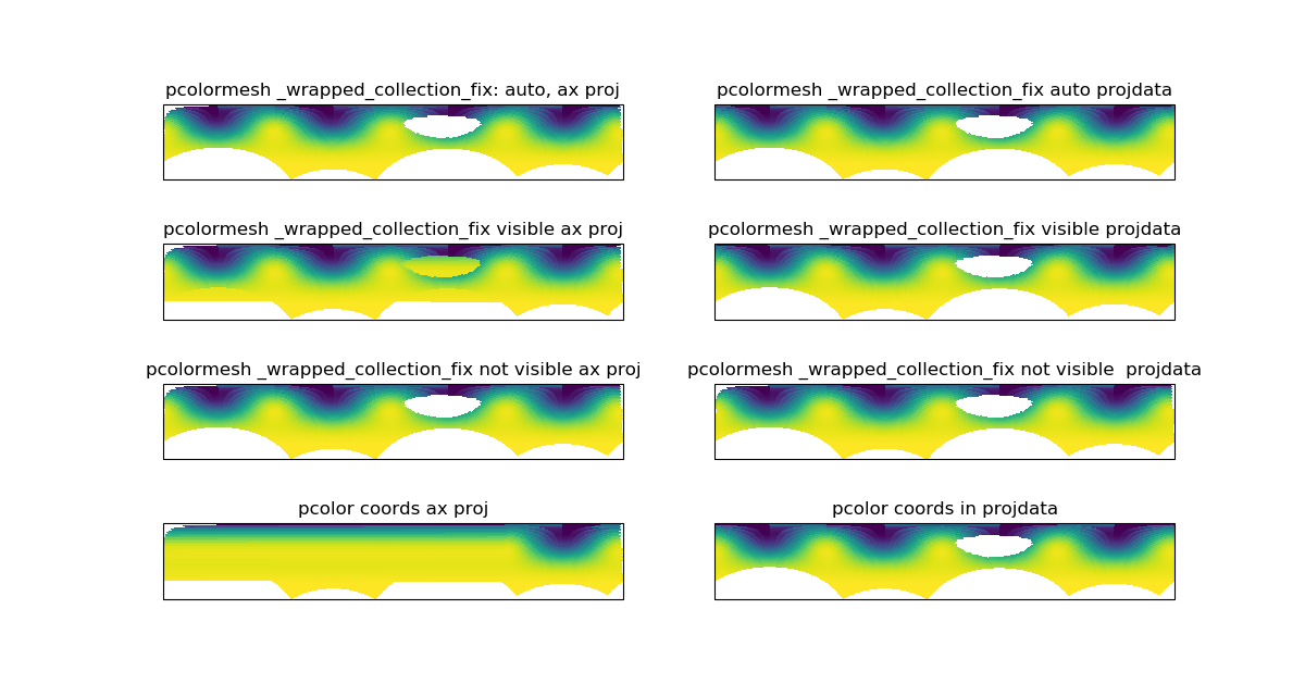
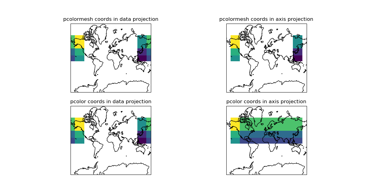
This PR is closed because taken into account by #1467 After further analysis and using both my example (ice data in stereographic projection) and the example above, I came to the conclusion that pcolor was failing to plot the overlapping cells when the data coordinates were given in the axis projection. Here is the code to used to show that point. Here is the resulting plot: Here is a very simple example with big cells showing how it works.
|
Commented out the part plotting the overlapping cells (despite a smaller zorder).
Now the overlapping cells larger than half the projection span stay masked.
Rationale
There is already a patch in pcolormesh that masks overlapping cells which are the cells crossing the longitude boundary and therefore overlapping the plot.
In that patch, the overlapping cells, those who size is more than half the projection span in x, are masked and plot then again with a zorder supposedly small enough so that they don't appear.
Unfortunately they still appeared on the plot.
The idea in plotting the bad cells is that someone may want to use them, by splitting them at the boundary and plot the split part. But they shouldn't be plotted as there are.
So the fix is to comment out the part plotting the bad cells.
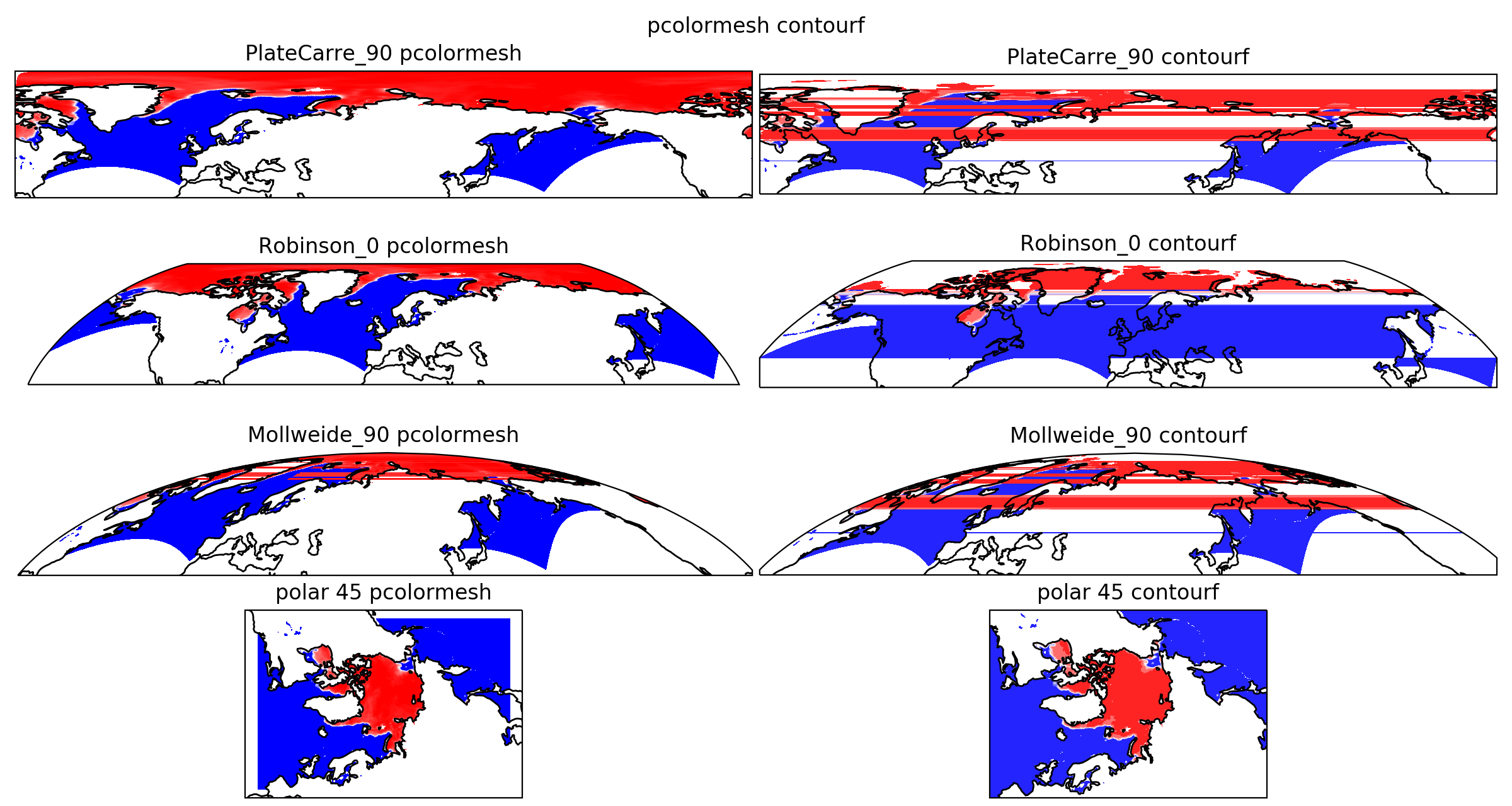
This patch works only for pcolormesh, there should be one of the same kind to mask the data generating overlapping cells or contours in contourf, pcolor and contour.
This patch removes the cell greater than half the projection span in x, which works well for Plate Carree but not for the narrow part of a projection like Mollweide. This part is not fixed.
The image below displays ice concentration provided in a polar stereographic grid.
It had been plotted after the proposed fix.
The left plots are pcolormesh which includes the patch for overlapping cells, the right plots are contourf and displays many overlapping cells.
The pcolormesh plot in Mollweide projection still displays some small overlapping cells (less than half the projection span) on the narrow part of the plot.
There are no overlapping cells in the stereographic projection.
The data can be found here.
Implications
I don't see any implication.