An implementation of Linear Regression from scratch in python 📈. Includes the hypothesis function, partial differentiation of variables, parameter update rule and gradient descent.
-
Download the project on your computer.
git clone https://github.com/sarvasvkulpati/LinearRegressionor download the ZIP file -
Go to the directory with the file:
cd LinearRegression -
Download the required packages:
pip install -r requirements.txt -
Run the project:
python3 LinearRegression.py
Linear regression is a method for approximating a linear relationship between two variables. While that may sound complicated, all it really means is that it takes some input variable, like the age of a house, and finds out how it's related to another variable, for example, the price it sells at.
We use it when the data has a linear relationship, which means that when you plot the points on a graph, the data lies approximately in the shape of a straight line.
Linear Regression involves a couple of steps:
- Randomly initialising parameters for the hypothesis function
- Computing the mean squared error
- Calculating the partial derivatives
- Updating the parameters based on the derivatives and the learning rate
- Repeating from 2 until the error is minimised
The linear equation is the standard form that represents a straight line on a graph, where m represents the gradient, and b represents the y-intercept.
The Hypothesis Function is the exact same function in the notation of Linear Regression.
The two variables we can change – m and b – are represented as parameters theta1 and theta0
In the beginning, we randomly initialize our parameters, which means we give theta1 and theta0 random values
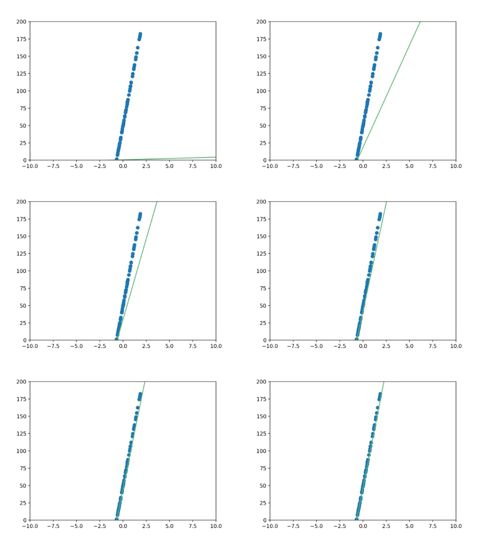
to begin with. This will output a random line, maybe something like this:

Clearly the line drawn in the graph above is wrong. But how wrong is it? That's what the error function is for - it calculates the total error of your graph. We'll be using an error function called the Mean Squared Error function, or MSE, represented by the letter J.
Now while that may look complicated, what it's doing is actually quite simple. The function J takes our parameters theta0, and theta1 as an input. Then, from every point from 1 to m, where m is the number of points, it calculates the distance between the x value and the value predicted by our function and squares it. Squaring it ensures that the error is always positive, and that the error is greater the further away the predicted value is from the actual value.
Now that we have a value for how wrong our function is, we need to adjust the function to reduce this error.
If we graph our parameters against the error (i.e graphing the cost function), we'll find that it forms something similar to the graph below. Our goal is to find the lowest point of that graph, where the error is at its lowest. This is called minimising the cost function.
To do this, we need to consider what happens at the bottom of the graph - the gradient is zero. So to minimize the cost function, we need to get the gradient to zero.
The gradient is given by the derivative of the function, and the partial derivatives of the functions are
Now we need to update our parameters to reduce the gradient. To do this, we use the gradient update rule
Alpha is what we call the Learning rate, which is a small number that allows the parameters to be updated by a small amount. As mentioned above, we are trying to update the gradient such that it's closer to zero (the bottom). The Learning rate helps guide the network to the lowest point on the curve by small amounts.
Now we repeat these steps - checking the error, calculating the derivatives, and updating the weights, until the error is as low as possible. This is called minimising the cost funtion.
Once your error is minimised, your line should now be the best possible fit to approximate the data!

