Vectorflow

Vectorflow is a tool designed for visualizing vector fields using a 2D field equation. It represents the velocity of each point in the field with a particle that traces a path. This project and guide draw inspiration from Anvaka's Fieldplay repository. The entire project is written in Rust and compiled to Web Assembly. Try it out on nyberg.dev/vectorflow/

What?

Let's assign to every point on a grid a vector (1, 0). This means we have an arrow, pointing to the right:

Let's pretend these vectors represent velocity. What if we drop a thousand particles onto this grid? How would they move?

When we assigned a vector to each point on the plain, we created a mathematical structure called Vector Field.

Let's create a bit more interesting vector field:

• Points with even y coordinate get vector (1, 0);
• Points with odd y coordinate get an opposite vector (-1, 0);

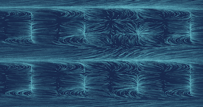
Again we drop a few thousands particles and see what happens:

The field above can be written in a single formula:

(
50 * (floor(y/100) % 2) - 25
,
0.0
)

The floor function effectively rounds down all y values to the nearest integer. As a result, the first 100 pixels assume the value 0, the subsequent 100 pixels take on the value 1, and so forth. By applying the modulo of 2 to these values, we obtain 0 for even numbers and 1 for odd numbers. We then manipulate this remainder to generate a final vector, which is either (-25, 0) or (25, 0).

Up until now, we've exclusively utilized one component of the velocity vector, specifically x, causing the particles to move solely horizontally. Let's experiment with configuring both components and observe the outcomes.

(
50 * (floor(y/100) % 2) - 25
,
50 * (floor(x/100) % 2) - 25
)

Wow! Two simple operations, and the final animation looks like an art piece!

Vector fields turns out to be very flexible generative framework.

Parser Syntax

The parser function utilizes the x and y coordinates as well as the distance from the origin r and the angle with the x-axis a of each pixel to compute the corresponding vector, it also has the ability to use the t variable to create time-dependent fields where t is measured in seconds, and resers every minute. Furthermore, it offers the following functionalities:

constants:
pi  // 3.141592653589793
e   // 2.718281828459045

variables:
x
y
t  // time in seconds
r  // distance from origin
a  // angle with the x-axis

Single variable functions:
sin(x)
cos(x)
tan(x)
sqrt(x)   // square root
abs(x)    // absolute value
sgn(x)    // signum function
floor(x)  // round down
ceil(x)   // round up

Two variable functions:
a + b
a - b
a * b
a / b
a ^ b  // power
a % b  // modulo
len(x1, y2, x2, y2)  // distance between two points

Cool Examples

Here are some cool example, feel free to suggest some yourself!

Dipole

(
x*y/1000
,
(y*y - x^2)/1000
)

Swirls

(
x+r * sin(sqrt(r))
,
y+r * cos(sqrt(len(x,x)))
)

Black Hole

(
y/(r^2/100000 - 0.001*x)
,
-x/(r^2/10000 - 0.001*y)
)

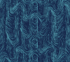
Mosaic

(
10*sin(y/100 + x/1000)*t
,
10*cos(x/100 - y/1000)*t
)

Eye

(
x*cos(abs(sin(t/4))*600/r) - y*sin(abs(sin(t/4))*600/r)
,
x*sin(abs(sin(t/4))*600/r) + y*cos(abs(sin(t/4))*600/r)
)

Radar

(
-y + (1-((x*sin(t) + y*cos(t))/abs(x*sin(t) + y*cos(t))))^10*x
,
x  + (1-((x*sin(t) + y*cos(t))/abs(x*sin(t) + y*cos(t))))^10*y
)