Detailed Design Document
-
Detailed Design
- 1 Process Flow Design
- 2 Algorithm Design
- 3 Class Design
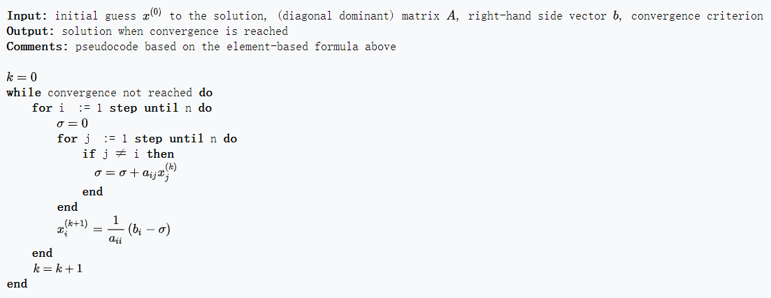
Jacobi method is an iterative algorithm for determining the solutions of a strictly diagonally dominant system of linear equations. Each diagonal element is solved for, and an approximate value is plugged in. The process is then iterated until it converges. This algorithm is a stripped-down version of the Jacobi transformation method of matrix diagonalization. The method is named after Carl Gustav Jacob Jacobi.
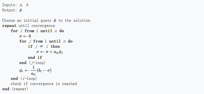
Gauss–Seidel method, also known as the Liebmann method or the method of successive displacement, is an iterative method used to solve a linear system of equations. It is named after the German mathematicians Carl Friedrich Gauss and Philipp Ludwig von Seidel, and is similar to the Jacobi method. Though it can be applied to any matrix with non-zero elements on the diagonals, convergence is only guaranteed if the matrix is either diagonally dominant, or symmetric and positive definite.
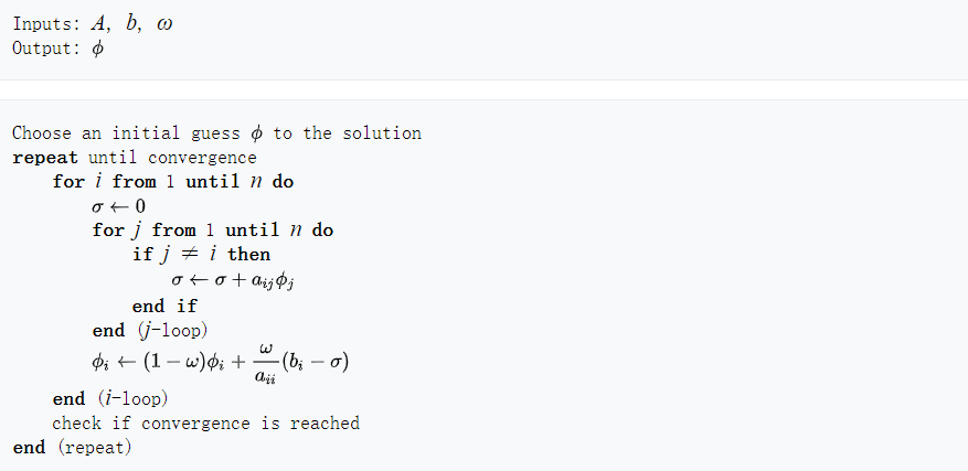
SOR method is a variant of the Gauss–Seidel method for solving a linear system of equations, resulting in faster convergence. A similar method can be used for any slowly converging iterative process. It was devised simultaneously by David M. Young, Jr. and by Stanley P. Frankel in 1950 for the purpose of automatically solving linear systems on digital computers. Convergence is only guaranteed if the matrix is either diagonally dominant, or symmetric and positive definite, which is the same as Gauss–Seidel method.
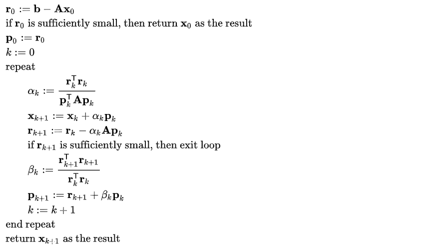
Conjugate gradient method is an algorithm for the numerical solution of particular systems of linear equations, namely those whose matrix is symmetric and positive-definite. The conjugate gradient method is often implemented as an iterative algorithm, applicable to systems that are too large to be handled by a direct implementation or other direct methods such as the Cholesky decomposition.
To solve a linear system of equations like
-
Rank of coefficient matrix n
-
Coefficient matrix
$A$ Convergence conditions must be meet. Input all elements of a sparse matrix in row-first order.
-
Vector
$b$ -
Solution precision
$p$ -
Output filename
$f$
Iteration continues until the error is less than pre-defined precision or iteration times is more than the upper limit.
- Iteration times
- Time costs
- Current error
- Solution
- Solution file
Let
$$
A \mathbf{x}=\mathbf{b}
$$
be a square system of
The computation of
The Gauss–Seidel method is an iterative technique for solving a square system of
Given a square system of
The method of successive over-relaxation is an iterative technique that solves the left hand side of this expression for
Suppose we want to solve the system of linear equations:
$$
A \mathbf{x}=\mathbf{b}
$$
for the vector
-
As a direct method
We say that two non-zero vectors
$\mathbf{u}$ and$\mathbf{v}$ are conjugate if $$ \mathbf{u}^{\top} \mathbf{A} \mathbf{v}=0 $$ Since$A$ is symmetric and positive-definite, the left-hand side defines an inner product: $$ \mathbf{u}^{\top} \mathbf{A} \mathbf{v}=\langle\mathbf{u}, \mathbf{v}\rangle_{\mathbf{A}}:=\langle\mathbf{A} \mathbf{u}, \mathbf{v}\rangle=\left\langle\mathbf{u}, \mathbf{A}^{\top} \mathbf{v}\right\rangle=\langle\mathbf{u}, \mathbf{A} \mathbf{v}\rangle $$ Two vectors are conjugate if and only if they are orthogonal with respect to this inner product. Being conjugate is a symmetric relation: if u is conjugate to v, then v is conjugate to u. Suppose that: $$ P=\left{\mathbf{p}{1}, \dots, \mathbf{p}{n}\right} $$ is a set of$n$ mutually conjugate vectors (with respect to$A$ ). Then$P$ forms a basis for$\mathbb{R}^{n},$ and we may express the solution $\mathbf{x}{*}$ of $A \mathbf{x}=\mathbf{b}$ in this basis: $$ \mathbf{x}{}=\sum_{i=1}^{n} \alpha_{i} \mathbf{p}{i} $$ Based on this expansion we calculate: $$ \mathbf{A} \mathbf{x}{}=\sum_{i=1}^{n} \alpha_{i} \mathbf{A} \mathbf{p}{i} $$ Left-multiplying by $\mathbf{p}{k}^{\top}$: $$ \mathbf{p}{k}^{\top} \mathbf{A} \mathbf{x}{}=\sum_{i=1}^{n} \alpha_{i} \mathbf{p}{k}^{\top} \mathbf{A} \mathbf{p}{i} $$ substituting $\mathbf{A} \mathbf{x}_{} = \mathbf{b}$ and$\mathbf{u}^{\top} \mathbf{A} \mathbf{v}=\langle\mathbf{u}, \mathbf{v}\rangle_{\mathbf{A}}$ : $$ \mathbf{p}{k}^{\top} \mathbf{b}=\sum{i=1}^{n} \alpha_{i}\left\langle\mathbf{p}{k}, \mathbf{p}{i}\right\rangle_{\mathbf{A}} $$ then$\mathbf{u}^{\top} \mathbf{v}=\langle\mathbf{u}, \mathbf{v}\rangle$ and using $\forall i \neq k:\left\langle\mathbf{p}{k}, \mathbf{p}{i}\right\rangle_{\mathbf{A}}=0$ yields: $$ \left\langle\mathbf{p}{k}, \mathbf{b}\right\rangle=\alpha{k}\left\langle\mathbf{p}{k}, \mathbf{p}{k}\right\rangle_{\mathbf{A}} $$ which implies: $$ \alpha_{k}=\frac{\left\langle\mathbf{p}{k}, \mathbf{b}\right\rangle}{\left\langle\mathbf{p}{k}, \mathbf{p}{k}\right\rangle{\mathbf{A}}} $$ This gives the following method for solving the equation$A \mathbf{x}=\mathbf{b}$ : find a sequence of$n$ conjugate directions, and then compute the coefficients$\alpha_{k}$ . -
As an iterative method
If we choose the conjugate vectors
$p_{k}$ carefully, then we may not need all of them to obtain a good approximation to the solution$\mathbf{x_{*}}$ . So, we want to regard the conjugate gradient method as an iterative method. This also allows us to approximately solve systems where n is so large that the direct method would take too much time.We denote the initial guess for $\mathbf{x_{}}$ by $\mathbf{x_{0}}$ (we can assume without loss of generality that $\mathbf{x_{0}}=0$, otherwise consider the system $\mathbf{Az} = \mathbf{b-Ax_{0}}$ instead). Starting with we $\mathbf{x_{0}}$search for the solution and in each iteration we need a metric to tell us whether we are closer to the solution $\mathbf{x_{}}$ that is known to us. This metric comes from the fact that the solution x∗ is also the unique minimizer of the following quadratic function: $$ f(\mathbf{x})=\frac{1}{2} \mathbf{x}^{\top} \mathbf{A} \mathbf{x}-\mathbf{x}^{\top} \mathbf{b}, \quad \mathbf{x} \in \mathbf{R}^{n} $$ The existence of a unique minimizer is apparent as its second derivative is given by a symmetric positive-definite matrix: $$ \nabla^{2} f(\mathbf{x})=\mathbf{A} $$ and that the minimizer solves the initial problem is obvious from its first derivative: $$ \nabla f(\mathbf{x})=\mathbf{A} \mathbf{x}-\mathbf{b} $$ This suggests taking the first basis vector
$p_{0}$ to be the negative of the gradient of f at$\mathbf{x=x_{0}}$ . The gradient of f equals$\mathbf{Ax-b}$ . Starting with an initial guess$\mathbf{x_{0}}$ , this means we take$\mathbf{p_{0}=b-Ax_{0}}$ . The other vectors in the basis will be conjugate to the gradient, hence the name conjugate gradient method. Note that$\mathbf{p_{0}}$ is also the residual provided by this initial step of the algorithm.Let
$\mathbf{r_{k}}$ be the residual at$k$ th step: $$ \mathbf{r}{k}=\mathbf{b}-\mathbf{A} \mathbf{x}{k} $$ As observed above,$\mathbf{r_{k}}$ is the negative gradient of f at$\mathbf{x=x_{k}}$ , so the gradient descent method would require to move in the direction$\mathbf{r_{k}}$ . Here, however, we insist that the directions$\mathbf{p_{k}}$ be conjugate to each other. A practical way to enforce this, is by requiring that the next search direction be built out of the current residual and all previous search directions. This gives the following expression: $$ \mathbf{p}{k}=\mathbf{r}{k}-\sum_{i<k} \frac{\mathbf{p}{i}^{\top} \mathbf{A} \mathbf{r}{k}}{\mathbf{p}{i}^{\top} \mathbf{A} \mathbf{p}{i}} \mathbf{p}{i} $$ Following this direction, the next optimal location is given by: $$ \mathbf{x}{k+1}=\mathbf{x}{k}+\alpha{k} \mathbf{p}{k} $$ with: $$ \alpha{k}=\frac{\mathbf{p}{k}^{\top}\left(\mathbf{b}-\mathbf{A} \mathbf{x}{k}\right)}{\mathbf{p}{k}^{\top} \mathbf{A} \mathbf{p}{k}}=\frac{\mathbf{p}{k}^{\top} \mathbf{r}{k}}{\mathbf{p}{k}^{\top} \mathbf{A} \mathbf{p}{k}} $$ where the last equality follows from the definition of$\mathbf{r_{k}}$ . The expression for$\alpha_{k}$ can be derived if one substitutes the expression for$\mathbf{x_{k+1}}$ into$f$ and minimizing it: $$ f\left(\mathbf{x}{k+1}\right)=f\left(\mathbf{x}{k}+\alpha_{k} \mathbf{p}{k}\right)=: g\left(\alpha{k}\right) $$$$ g^{\prime}\left(\alpha_{k}\right) \stackrel{!}{=} 0 \quad \Rightarrow \quad \alpha_{k}=\frac{\mathbf{P}{k}^{\top}\left(\mathbf{b}-\mathbf{A} \mathbf{x}{k}\right)}{\mathbf{p}{k}^{\top} \mathbf{A} \mathbf{p}{k}} $$
Of the above four algorithms, each iteration of the Gauss-Seidel method and SOR method requires the results of the previous iteration, so there is not much parallelism that can be mined. In fact, their improvement ideas for Jacobi method have included the digging of their parallelism. We focus on the iterative implementation of Jacobi method and Conjugate gradient method.
-
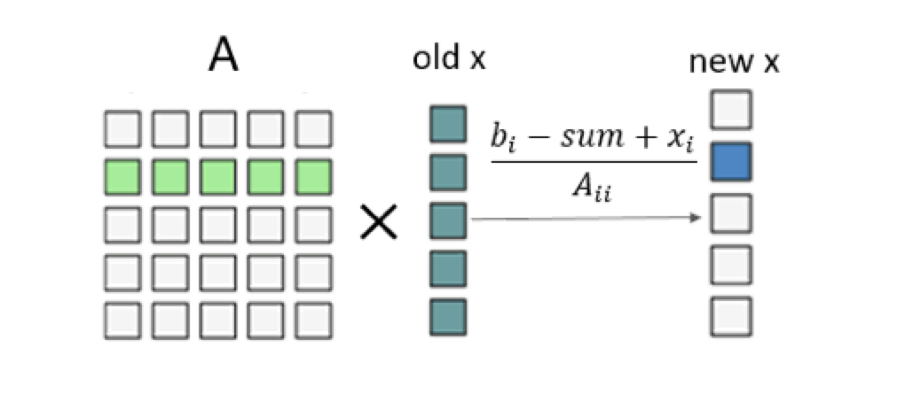
Idea: Set the grid to a one-dimensional grid that contains several thread blocks. Each thread block is also set to a one-dimensional form, which contains several threads. Each of these threads is responsible for calculating one element of
$x$ in each round of iteration, that is, to calculate a row in A by$x$ (one column) in a loop traversal step of 1.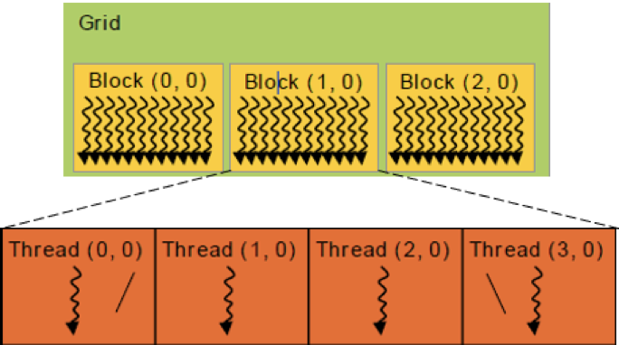
-
Analysis:
- Advantage: The serial calculation is transformed into the parallel calculation, thereby reducing the time cost through basic parallel acceleration.
-
Disadvantage: The thread in each thread block will access the data located in the global memory multiple times, that is, the x of the previous iteration. The calculation of a row of
$x$ and a column of$A$ is performed by only one thread. The single thread is overburdened, the parallelism is not high enough, and the efficiency is too low.
-
Idea: In view of the problems in the above method, we change the step size of the loop traversal calculation form 1 to the thread block size. At the same time, a shared memory array with the same size as the thread block is set for each thread block, and then each thread in a thread block in a round loop will load one element in a shared memory array in parallel. Thus
$x$ in global memory only needs to be accessed once per round. After that,$x$ can be read from the shared memory.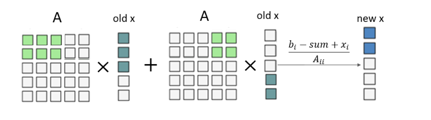
-
Analysis:
- Advantage: The statements in the loop unrolling are not data related, increasing the chance of concurrent execution. Most of the reads from global memory will be replaced by faster shared block memory, which will reduce the memory data read consumption.
- Disadvantage: The calculation of the next x element is still completed by only one thread, so its parallelism is still not high enough.
-
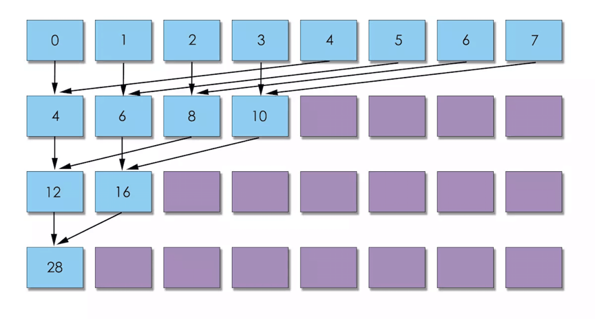
Idea: To solve the above problem, the grid is still set to one dimension, but its length is set to be equal to the number of rows of the coefficient matrix. The size of each thread block is set to 32, which is consistent with the size of the thread unit SM execution basic unit thread bundle in the GPU. Threads in a thread block are responsible for multiplying a row in A by an x (a column). Each thread multiplies the 32 in a row of A and accumulates them. Each thread adds and accumulates in parallel to their respective endpoints, and then sums the reductions among the 32 threads through Warp Shuffle.
-
Analysis:
- Advantage: The calculation of an x element is shared by 32 threads. At the same time, the loading of one row of A and the data of x (the previous one) is also jointly responsible for these 32 threads, which increases the parallelism. Reduce the number of additions by using the convention to further sum up the cumulative sum of $ 32 $ threads. Warp Shuffle is used to allow threads to directly read the register values of other threads in the same thread bundle, with very low latency, and without consuming additional memory resources to perform data exchange.
Basic CUDA parallelism acceleration and shared memory are both applied in conjugate gradient method.
For many large-scale computer simulation and analysis tasks, it is sparse linear systems that account for most of the computing time and resources in computing. For example, using the finite element method for structural static analysis, the solution of sparse linear equations usually accounts for more than 80% of the entire time overhead. In the field of engineering and scientific research, the complexity of the problem is getting higher and higher, and the scale is getting larger and larger, which leads to the increasing scale of solving sparse linear systems, and at the same time, there are higher requirements on the calculation speed. The use of high performance and parallel computing technology is an important way to solve large sparse linear systems.
Conjugate gradient method is applicable to sparse systems that are too big to be handled by a direct implementation. In this method, due to the memory limit, sparse matrix storage strategy needs considering.
To solve a linear system of equations like
-
Rank of coefficient matrix n
-
The number of non-zero elements of coefficient matrix
$count$ -
Coefficient matrix
$A$ Convergence conditions must be meet. Coefficient matrix
$A$ must be input in CSR format which is from the index pointer arrays to the index array to value array. -
Vector
$b$ -
Solution precision
$p$ -
Output filename
$f$
Iteration continues until the error is less than pre-defined precision or iteration times is more than the upper limit.
- Iteration times
- Time costs
- Current error
- Solution
- Solution file
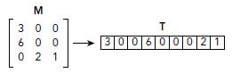 Fig 2-1. Dense Format Fig 2-1. Dense Format
|
 Fig 2-2. Coordinate (COO) Fig 2-2. Coordinate (COO)
|
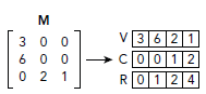 Fig 2-3. Compressed Sparse Row (CSR) Fig 2-3. Compressed Sparse Row (CSR)
|
Use cuSPARSE to implement data conversion.

The cuSOLVER library is a high-level package based on the cuBLAS and cuSPARSE libraries. It consists of two modules corresponding to two sets of API:
- The cuSolver API on a single GPU
- The cuSolverMG API on a single node multiGPU
Each of which can be used independently or in concert with other toolkit libraries. To simplify the notation, cuSolver denotes single GPU API and cuSolverMg denotes multiGPU API.
The intent of cuSolver is to provide useful LAPACK-like features, such as common matrix factorization and triangular solve routines for dense matrices, a sparse least-squares solver and an eigenvalue solver. In addition cuSolver provides a new refactorization library useful for solving sequences of matrices with a shared sparsity pattern.
- Read the sparse coefficient matrix from the file and use the sparse matrix storage format in the cuSPARSE library to convert to the CSR storage format.
- Then in each step of the conjugate gradient method, the part involving the sparse coefficient matrix is directly calculated using the function in the cuSPARSE library (such as cusparseScsrmv), and the operation that does not involve the sparse matrix uses the function of cuBLAS (such as cublasSaxpy, cublasSdot).
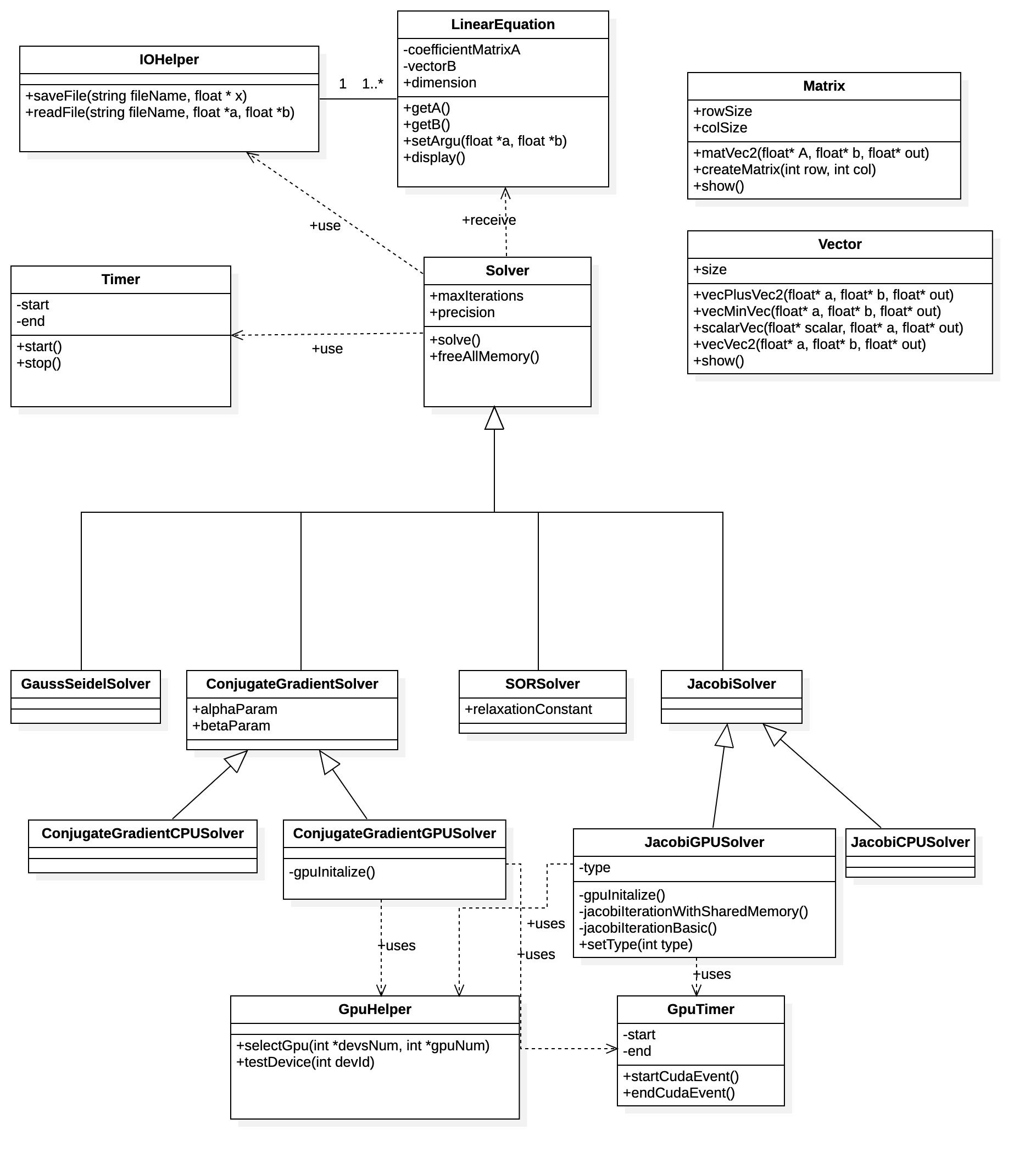
The following diagram is the total class diagram, followed with a class description of each class.
public class LinearEquation
Description:To store linear equation.
Fields
| Modifier and Type | Field | Description |
|---|---|---|
| private float * | coefficientMatrixA | coefficient matrix A in |
| private float * | vectorB | vector b in |
| public int | dimension | the size of vector b |
Methods
| Main Method | Access right | Return | Description |
|---|---|---|---|
| getA() | public | private float * | get coefficient matrix A |
| getB() | public | private float * | get vector b |
| setArgu(float * a, float * b) | public | void | set coefficient matrix A and vector b |
| display() | public | void | print coefficient matrix A and vector b |
public class IOHelper
Description:To read and save equation parameters.
Fields
none
Methods
| Main Method | Access right | Return | Description |
|---|---|---|---|
| saveFile(string fileName, float * x) | public | void | save result x in |
| readFile(string fileName, float *a, float *b) | public | void | read A and b in |
public class Timer
Description:To count time.
Fields
| Modifier and Type | Field | Description |
|---|---|---|
| private clock_t | start | the timer start time |
| private clock_t | end | the timer stop time |
Methods
| Main Method | Access right | Return | Description |
|---|---|---|---|
| start() | public | void | to start the timer |
| stop() | public | float | to stop timer and return time interval |
public class Solver
Description:To solve linear equation.
Fields
| Modifier and Type | Field | Description |
|---|---|---|
| private int | maxIterations | the limitation of max iteraton |
| private float | precision | the precision of result x in |
Methods
| Main Method | Access right | Return | Description |
|---|---|---|---|
| freeAllMemory() | public | void | to free all memory that allocated in the process of solving |
| solve | public | void | to solve the equation |
public class Timer
Description:To count time.
Fields
| Modifier and Type | Field | Description |
|---|---|---|
| private double | start | the time when the cuda event start |
| private double | end | the time when the cuda event end |
Methods
| Main Method | Access right | Return | Description |
|---|---|---|---|
| startCudaEvent() | public | void | to start the cudaEventTimer |
| stopCudaEvent() | public | double | to stop cudaEvent and return time interval |
public class GpuHelper
Description:To help test gpus and select best gpu.
Fields
none
Methods
| Main Method | Access right | Return | Description |
|---|---|---|---|
| selectGpu(int *devsNum, int *gpuNum) | public | void | to save the num of best gpu to gpuNum |
| testDevice(int devId) | public | void | to test whether the gpu with id devId is supporting cuda |
public class SORSolver extends Solver
Description:To solve linear equation by SOR.
Fields
| Modifier and Type | Field | Description |
|---|---|---|
| public float | relaxationConstant | the relaxation constant for SOR method |
public class ConjugateGradientSolver extends Solver
Description:To solve linear equation by ConjugateGradient.
Fields
| Modifier and Type | Field | Description |
|---|---|---|
| public float | alphaParam | the alpha parameter for ConjugateGradient method |
| public float | betaParam | the beta parameter for ConjugateGradient method |
public class **JacobiGPUSolver **extends JacobiSolver
Description:To solve linear equation with jacobi method in gpu .
Fields
| Modifier and Type | Field | Description |
|---|---|---|
| private int | type | the type of jacobi method implemted in GPU |
Methods
| Main Method | Access right | Return | Description |
|---|---|---|---|
| gpuInitalize() | public | void | to initialize cuda environment |
| jacobiIterationWithSharedMemory() | public | void | to do iterations in gpu with sharememory |
| jacobiIterationBasic() | public | void | to do iterations in gpu with basic method |
| setType(int type) | public | void | set the type of jacobi implements |
public class **ConjugateGradientGPUSolver **extends ConjugateGradientSolver
Description:To solve linear equation with ConjugateGradient method in gpu .
Fields
none
Methods
| Main Method | Access right | Return | Description |
|---|---|---|---|
| gpuInitalize() | public | void | to initialize cuda environment |
Software Engineering, Fall 2019 & Software Test, Spring 2020.
It is a collaborative and interdisciplinary project drawing on expertise from School of Software Engineering & College of Civil Engineering, Tongji University.

