Yields.jl provides a simple interface for constructing, manipulating, and using yield curves for modeling purposes.
It's intended to provide common functionality around modeling interest rates, spreads, and miscellaneous yields across the JuliaActuary ecosystem (though not limited to use in JuliaActuary packages).
using Yields

riskfree_maturities = [0.5, 1.0, 1.5, 2.0]
riskfree    = [5.0, 5.8, 6.4, 6.8] ./ 100     #spot rates, annual effective if unspecified

spread_maturities = [0.5, 1.0, 1.5, 3.0]      # different maturities
spread    = [1.0, 1.8, 1.4, 1.8] ./ 100       # spot spreads

rf_curve = Yields.Zero(riskfree,riskfree_maturities)
spread_curve = Yields.Zero(spread,spread_maturities)


yield = rf_curve + spread_curve               # additive combination of the two curves

discount(yield,1.5) # 1 / (1 + 0.064 + 0.014) ^ 1.5Rates are types that wrap scalar values to provide information about how to determine discount and accumulation factors.
There are two CompoundingFrequency types:
Yields.Periodic(m)for rates that compoundmtimes per period (e.g.mtimes per year if working with annual rates).Yields.Continuous()for continuously compounding rates.
Continuous(0.05)       # 5% continuously compounded
Periodic(0.05,2)       # 5% compounded twice per period
These are both subtypes of the parent Rate type and are instantiated as:
Rate(0.05,Continuous())       # 5% continuously compounded
Rate(0.05,Periodic(2))        # 5% compounded twice per period
Broadcast over a vector to create Rates with the given compounding:
Periodic.([0.02,0.03,0.04],2)
Continuous.([0.02,0.03,0.04])
Rates can also be constructed by specifying the CompoundingFrequency and then passing a scalar rate:
Periodic(1)(0.05)
Continuous()(0.05)Convert rates between different types with convert. E.g.:
r = Rate(Yields.Periodic(12),0.01)             # rate that compounds 12 times per rate period (ie monthly)

convert(Yields.Periodic(1),r)                  # convert monthly rate to annual effective
convert(Yields.Continuous(),r) # convert monthly rate to continuousAdding, substracting, multiplying, dividing, and comparing rates is supported.
There are a several ways to construct a yield curve object. If maturities is omitted, the method will assume that the timepoints corresponding to each rate are the indices of the rates (e.g. generally one to the length of the array for standard, non-offset arrays).
There is a set of constructor methods which will return a yield curve calibrated to the given inputs.
Yields.Zero(rates,maturities)using a vector of zero rates (sometimes referred to as "spot" rates)Yields.Forward(rates,maturities)using a vector of forward ratesYields.Par(rates,maturities)takes a series of yields for securities priced at par. Assumes that maturities <= 1 year do not pay coupons and that after one year, pays coupons with frequency equal to the CompoundingFrequency of the corresponding rate (2 by default).Yields.CMT(rates,maturities)takes the most commonly presented rate data (e.g. Treasury.gov) and bootstraps the curve given the combination of bills and bonds.Yields.OIS(rates,maturities)takes the most commonly presented rate data for overnight swaps and bootstraps the curve. Rates assume a single settlement for <1 year and quarterly settlements for 1 year and above.
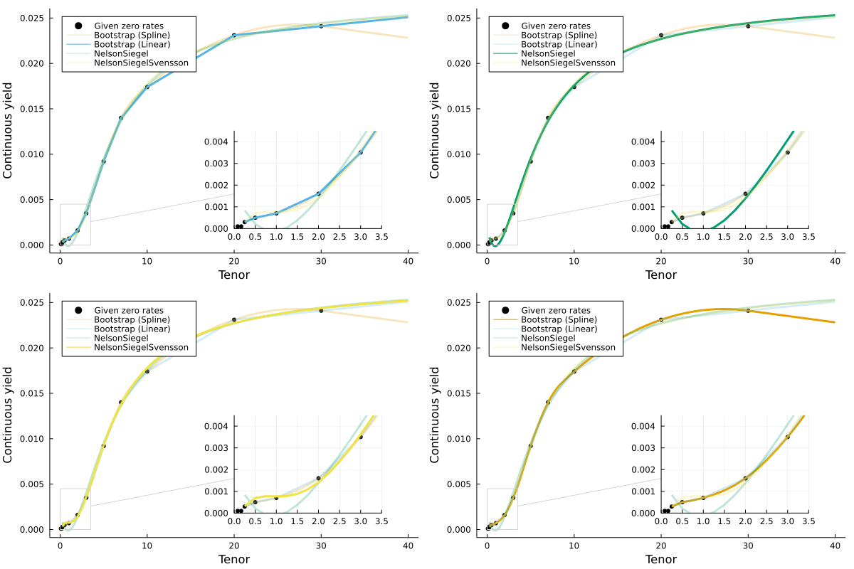
There are multiple curve fitting methods available:
Boostrap(interpolation_method)(the default method)- where
interpolationcan be one of the built-inQuadraticSpline()(the default) orLinearSpline(), or a user-supplied function.
- where
- Two methods from the Nelson-Siegel-Svensson family, where τ_initial is the starting τ point for the fitting optimization routine:
NelsonSiegel(τ_initial=1.0)NelsonSiegelSvensson(τ_initial=[1.0,1.0])
To specify which fitting method to use, pass the object to as the first parameter to the above set of constructors, for example: Yields.Par(NelsonSiegel(),rates,maturities).
Yields.SmithWilsoncurve (used for discounting in the EU Solvency II framework) can be constructed either directly by specifying its inner representation or by calibrating to a set of cashflows with known prices.- These cashflows can conveniently be constructed with a Vector of
Yields.ZeroCouponQuotes,Yields.SwapQuotes, orYields.BulletBondQuotes.
- These cashflows can conveniently be constructed with a Vector of
Yields.Constant(rate)takes a single constant rate for all timesYields.Step(rates,maturities)doesn't interpolate - the rate is flat up to the corresponding time intimes
Most of the above yields have the following defined (goal is to have them all):
discount(curve,from,to)ordiscount(curve,to)gives the discount factoraccumulation(curve,from,to)oraccumulation(curve,to)gives the accumulation factorzero(curve,time)orzero(curve,time,CompoundingFrequency)gives the zero-coupon spot rate for the given time.forward(curve,from,to)gives the zero rate between the two given timespar(curve,time)gives the coupon-paying par equivalent rate for the given time.
Different yield objects can be combined with addition or subtraction. See the Quickstart for an example.
When adding a Yields.AbstractYield with a scalar or vector, that scalar or vector will be promoted to a yield type via Yield(). For example:
y1 = Yields.Constant(0.05)
y2 = y1 + 0.01 # y2 is a yield of 0.06Constructed curves can be shifted so that a future timepoint becomes the effective time-zero for a said curve.
julia> zero = [5.0, 5.8, 6.4, 6.8] ./ 100
julia> maturity = [0.5, 1.0, 1.5, 2.0]
julia> curve = Yields.Zero(zero, maturity)
julia> fwd = Yields.ForwardStarting(curve, 1.0)

julia> discount(curve,1,2)
0.9275624570410582

julia> discount(fwd,1) # `curve` has effectively been reindexed to `1.0`
0.9275624570410582Generally, CamelCase methods which construct a datatype are exported as they are unlikely to conflict with other parts of code that may be written. For example, rate is un-exported (it must be called with Yields.rate(...)) because rate is likely a very commonly defined variable within actuarial and financial contexts and there is a high risk of conflicting with defined variables.
Consider using import Yields which would require qualifying all methods, but alleviates any namespace conflicts and has the benefit of being explicit about the calls (internally we prefer this in the package design to keep dependencies and their usage clear).
For time-variant yields (ie yield curves), the inputs are converted to spot rates and interpolated using quadratic B-splines by default (see documentation for alternatives, such as linear interpolations).
Combinations track two different curve objects and are not combined into a single underlying data structure. This means that you may achieve better performance if you combine the rates before constructing a Yields representation. The exception to this is Constant curves, which do get combined into a single structure that is as performant as pre-combined rate structure.
InterestRates.jlspecializes in fast rate calculations aimed at valuing fixed income contracts, with business-day-level accuracy.- Comparative comments:
Yields.jldoes not try to provide as precise controls over the timing, structure, and interpolation of the curve. Instead,Yields.jlprovides a minimal, but flexible and intuitive interface for common modeling needs.
- Comparative comments:


