
🖥️ Click me to see the dashboard ✨
Group 2: Paul Hübner, Jonas Müller
Topic: Predict weather-based public transport delays in Gävleborg.
When snowfall catches a city off-guard -- as it did in Munich in 2023 -- there are often drastic consequences for the public. Public transportation is shut down, flights are canceled, and big events postponed [1]. Gävleborg county sees snow quite frequently, and therefore should in theory be prepared in terms of infrastructure and operations. However, delays or cancellations still occur in public transportation [2]. Therefore, the goal of this project is to investigate to what extent a machine learning model can quantify delays. The purpose of the project is to aid the citizens of Gävleborg with a free online tool that they can then use in their own planning.
At the core of the project, there are two data sources:
- The traffic data from Trafiklab provides real-time and historical information on X-Trafik (Gävleborgs transit authority) and many other regional Swedish transit authorities. Data is collected both from the KoDa API (historical data) and the GTFS-Regional API (live data).
- The weather API from Open-Meteo is self-explanatory.
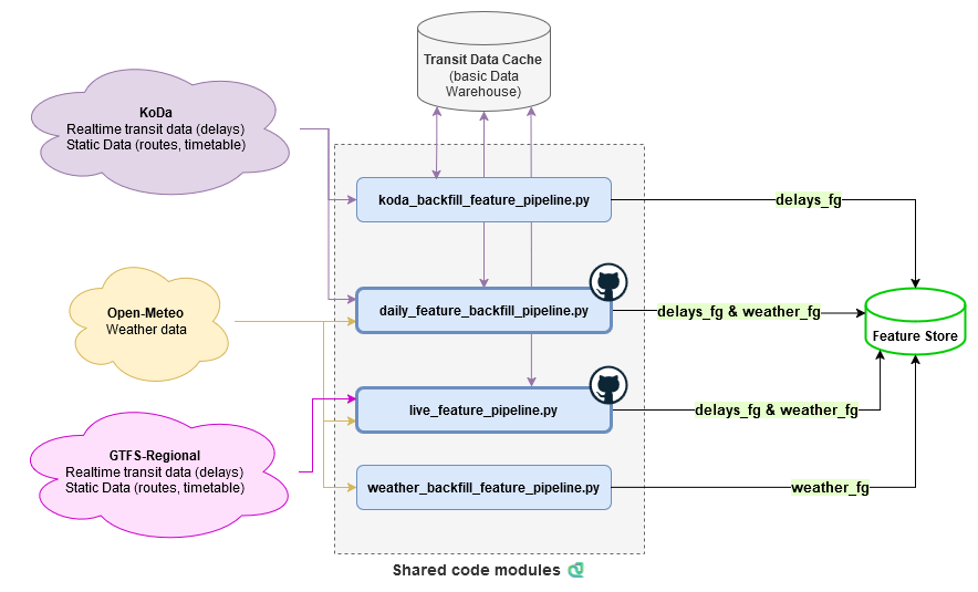
Backfills were executed on-demand, while daily and live feature pipelines run on GitHub Actions.
Overall, in the end, there were ~12 000 hourly datapoints available (limited by the historical X-Trafik data) of which we collected ~8 400 feature instances (rows in the feature view).
Below is more information on the different datasets used from these data sources, as well as their related scripts.
Transit operations data can be accessed in many different ways, but as having access to historical data was a priority for us, we decided to base our delay features on what the KoDa API could provide. While most transit APIs provide only real-time data which is updated and overwritten every few minutes, KoDa is unique in that it allows historical queries and returns a collection of 15-second snapshots of the realtime data for a day.
This data is structured in the GTFS format, but the snapshots needed to be merged and cleaned to be useful features.
Additionally, any features we created from the historical data also needed to be created from real-time data (GTFS-Regional API) for our inference pipeline.
To make this process easier, we created reusable data processing modules and functions, so the historical and live pipelines share
multiple parts of their code (chiefly the feature transformations in shared/features).
Note: The earliest tested successful historical request for operator xt was for 2022-02-01
- Purpose: Provide a backfill of data that can be used for model training.
- Source: KoDa
- Pipeline:
koda_backfill_feature_pipeline.py
Usage
Enviornment variables:
START_DATE: Start date for backfillingEND_DATE: End date for backfillingSTRIDE: Stride for backfillingDRY_RUN: If set toTrue, no data will be written to the feature store, only one day processed and written to a csv fileKODA_KEY: API key for KoDaUSE_PROCESSES: Number of processes to use for parallel processingHOPSWORKS_API_KEY: API key for HopsworksFG_VERSION: Version of the delay feature group to useRUN_HW_MATERIALIZATION_EVERY: How often to run Hopsworks materialization jobs in days processed
Example command: HOPSWORKS_API_KEY=your_key KODA_KEY=your_key USE_PROCESSES=4 START_DATE=2024-11-01 END_DATE=2024-11-01 STRIDE=4 DRY_RUN=False python3 koda_backfill_feature_pipeline.py
- Purpose: Provide ground-truth data for the previous day and keep building training collection.
- Source: KoDa
- Pipeline:
daily_feature_backfill_pipeline.py(Scheduled in.github/workflows/daily-backfill.yml)
Usage
Enviornment variables:
DRY_RUN: If set toTrue, no data will be written to the feature store, only output as csvsWEATHER_FG_VERSION: Version of the weather feature group to useDELAYS_FG_VERSION: Version of the delay feature group to useKODA_KEY: API key for KoDaUSE_PROCESSES: Number of processes to use for parallel processingHOPSWORKS_API_KEY: API key for Hopsworks
Example: WEATHER_FG_VERSION=1 HOPSWORKS_API_KEY=your_key DRY_RUN=False KODA_KEY=your_key python3 daily_feature_backfill_pipeline.py
- Purpose: Provide real-time data that can be used to make real-time delay predictions (
inference_pipeline.py). In reality, this is used in (at least) hourly batch inference, as opposed to truly real-time. - Source: GTFS-Regional
- Pipeline:
live_feature_pipeline.py(Scheduled in.github/workflows/regular-update.yml)
Usage
Enviornment variables:
DRY_RUN: If set toTrue, no data will be written to the feature store, only one day processed and written to a csv fileGTRFSR_RT_API_KEY: API key for GTFS Regional RealtimeGTRFSR_STATIC_API_KEY: API key for GTFS Regional StaticUSE_PROCESSES: Number of processes to use for parallel processingHOPSWORKS_API_KEY: API key for Hopsworks
Example: HOPSWORKS_API_KEY=your_key DRY_RUN=False python3 live_feature_pipeline.py
More information on the source data can be found here: https://open-meteo.com/en/docs.
Historical Backfill:
- Purpose: Provide a backfill of data that can be used for model training.
- Source: Archive API
- Pipeline:
weather_backfill_feature_pipeline.py
Usage
Enviornment variables:
START_DATE: Start date for backfillingEND_DATE: End date for backfillingHOPSWORKS_API_KEY: API key for HopsworksDRY_RUN: If set toTrue, no data will be written to the feature store, only one day processed and written to a csv file
Example: HOPSWORKS_API_KEY=your_key DRY_RUN=False START_DATE=2024-10-01 END_DATE=2024-11-01 python3 weather_backfill_feature_pipeline.py
Daily Backfill:
- Purpose: Provide ground-truth data for the previous day and keep building training collection.
- Source: Forecast API but for the previous day (Archive API does not provide short-term history).
- Pipeline:
daily_feature_backfill_pipeline.py(same as for delays)
Predictions
- Purpose: Provide (predicted) weather data for the future that can be used to make delay predictions (
inference_pipeline.py). - Source: Forecast API
- Pipeline:
live_feature_pipeline.py(same as for delays)
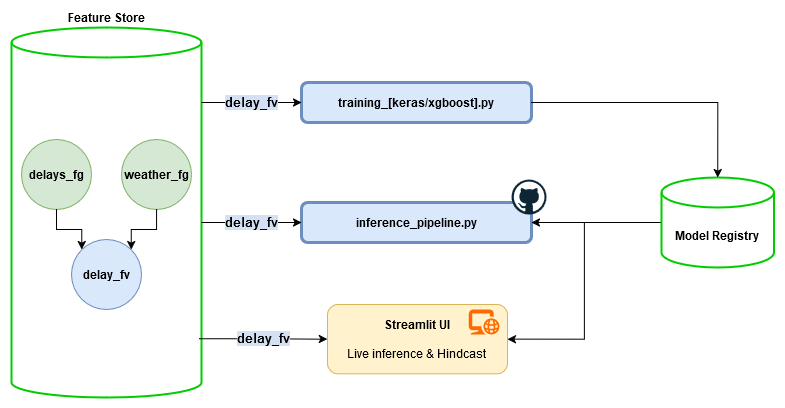
Both data sources provide a plethora of information. There are two feature groups, delays (via X-Trafik data) and weather.
The table below summarizes all the features. Which features to include in the final models was decided through trial and error early on. It was found that, as expected, too many features caused quite extreme overfitting. We ended up predicting two key labels, average arrival delay and on time percentage, and only using a subset of our total features as inputs.
All features are stored in the Hopsworks feature store for batch and online tasks.
All features (very long table)
| Group | Name | Type | Label | Used in model |
|---|---|---|---|---|
| Delays | route_type |
enum | ✅ | |
| Delays | arrival_time_bin |
timestamp | ✅ | |
| Delays | mean_delay_change_seconds |
double | ✅ | |
| Delays | max_delay_change_seconds |
double | ✅ | |
| Delays | min_delay_change_seconds |
double | ✅ | |
| Delays | var_delay_change_seconds |
double | ✅ | |
| Delays | mean_arrival_delay_seconds |
double | ✅ | |
| Delays | max_arrival_delay_seconds |
double | ✅ | |
| Delays | min_arrival_delay_seconds |
double | ✅ | |
| Delays | var_arrival_delay |
double | ✅ | |
| Delays | mean_departure_delay_seconds |
double | ✅ | |
| Delays | max_departure_delay_seconds |
double | ✅ | |
| Delays | min_departure_delay_seconds |
double | ✅ | |
| Delays | var_departure_delay |
double | ✅ | |
| Delays | mean_on_time_percent* |
double | ✅ | |
| Delays | mean_final_stop_delay_seconds |
double | ✅ | |
| Delays | mean_arrival_delay_seconds_lag_5stops |
double | ✅ | |
| Delays | mean_departure_delay_seconds_lag_5stops |
double | ||
| Delays | mean_delay_change_seconds_lag_5stops |
double | ||
| Delays | stop_count** |
double | ✅ | |
| Delays | trip_update_count |
integer | ||
| Weather | date |
timestamp | ||
| Weather | temperature_2m |
float | ✅ | |
| Weather | apparent_temperature |
float | ||
| Weather | precipitation |
float | ||
| Weather | rain |
float | ||
| Weather | snowfall |
float | ✅ | |
| Weather | snow_depth |
float | ✅ | |
| Weather | cloud_cover |
float | ||
| Weather | wind_speed_10m |
float | ||
| Weather | wind_speed_100m |
float | ||
| Weather | wind_gusts_10m |
float | ✅ | |
| Weather | hour |
int | ✅ |
*A train is considered on-time if it arrives no earlier than 3 minutes and no later than 5 minutes.
**An integer, just stored as a double for legacy reasons.
Of the available real-time data we exclusively used TripUpdates in combination with static GTFS data to gather context information such as planned stop count per hour
and route_type (bus or train).
To limit the project scope, we decided to focus on system-wide delays instead of individual vehicle or route metrics.
As such, when engineering features we aggregated delays across all routes and vehicles.
Additionally, knowing that weather data more granular than hourly would not be available, we decided to aggregate delays on an hourly basis.
This was accomplished by first merging all TripUpdate snapshots for a day, removing duplicates and then keeping only the latest update for each trip and stop,
leaving us with the most recent delay information for each stop of the day.
After calculating stop-level features, the stop-rows were grouped by route type and resampled into hourly bins.
In order to nevertheless capture temporal dependencies in the data, we experimented extensively with lagged features and sliding windows as well as
establishing other temporal features such as delay_change.
However, just using lagged arrival delays were found to be the most effective for our final prediction task.
ℹ️️ This hourly binning and lagging of features unfortunately also means that real-time predictions are more limited by how many and how early
TripUpdatesare published for future stops, as too few updates per hour would result in skewed aggregated features.
We also experimented with what labels would be most interesting to predict before settling on average delay and on-time percentage.
While weather is a regional phenomenon, we decided to only use weather data from Gävle, the capital of Gävleborg. We deemed this simplification reasonable as much of the X-Trafik routes are centered around Gävle and aggregating weather data for each stop location individually would likely not yield much additional information for system-wide delays on top of being complex to implement.
Our weather features are transformed very little.
We first selected all available features which could plausibly have an effect on delays before narrowing it down to temperature, snow and wind gusts.
We merely added the hour bin to the data in order to merge it with the delay features more easily.
Our methodology is an iterative empirical one. We performed the following:
- Download a part of the data (using strides, so every X days).
- Experiment with some models, play around with hyperparameters, try to develop good models.
- Perform a rigorous evaluation in the form of a grid search to get an understanding of how the models behave overall.
- Return to step 1.
At the same time, we worked on refining the data that we had. Additionally, we developed the UI as it was important to be able to see the data visually too.
We decided to develop two models, so that we could evaluate which one performed better in hyperparameter tuning. A brief description of the model is given below.
A decision tree using XGBoosts's XGBRegressor.
The XGBoost model is able to capture nonlinear relationships, and in our experience has performed well.
Therefore, it is worth investigating, especially since it is computationally cheap to train.
An artificial neural network using keras and tensorflow.
ANNs can learn extremely complex relationships.
While we were unsure if there was enough data, we decided it was definitely worth investigating.
The final (hyperparameter tuned) ANN had one hidden layer of size 16.
The ANN network diagram

This section very crudely outlines how the models were trained. Trained models were saved on Hopsworks in the model registry.
In order to start with training, model-specific preprocessing had to be performed on the features. The route type feature had to be one-hot encoded, but other than that the features were mostly already clean.
From all available data, a training dataset was created on Hopsworks. One of the challenges was to determine how to split this set into training and test sets. There were two options:
- Dedicate every X datapoints to the test set. Make the cycle such that the test set sees various weekdays, seasons, etc.
- Use every day after day X as a test day and train on the days before.
We ended up going with the second option. While the first seemed to make more sense intuitively, it was not performing as well. Similarly, once lagged data was added, this was kind of cheating, as some training days had the lagged value of test days. Since we had almost 3 years worth of data, this would ensure that there was sufficient season data available in the training set. The test set was everything after Midsommar 2024 (2024-06-22).
For the ANN, normalization of the inputs/outputs was required.
For this, we used sklearn.
StandardScaler was found to outperform MinMaxScaler, MaxAbsScaler and (surprisingly) RobustScaler.
The scaler mean/variance was attached to the TensorFlow model as a variable and uploaded to Hopsworks.
The files training_keras.py and training_xgboost.py provided workbenches to quickly train and iterate over models.
One caveat is that training data must reside locally on the computer, to avoid the Hopsworks delays.
As aforementioned, the features were narrowed down using trial and error. For the ANN, 40 epochs of 32 batch sizes seemed to provide the best results.
We performed a grid search on the models. The training dataset was first split into a train and test set. The test set was withheld entirely, and the training set used in a 5-fold cross validation set. This then randomly produced training and validation features and labels.
The hyperparameters that were trialled were:
xgboost_grid = {
    "learning_rate": [0.1, 0.2, 0.3, 0.4],
    "max_depth": [2, 4, 6, 8]
}

keras_grid = {
    "model__lr": [0.001, 0.005, 0.1],
    "model__hidden": [8, 10, 16, 32],
    "model__activation": ["relu", "sigmoid", "tanh"],
}
Hyperparameter tuning took at most a minute for the decision tree. The rest of the many hours spent training were spent on tuning the ANN.
In order to evaluate our models numerically, we chose to use R². We find this to be a more interpretable than MSE.
The best models on the final dataset were as follows:
| Model | Hyperparameters | R² |
|---|---|---|
| Decision Tree | learning rate: 0.2, max depth: 4 | 0.37 |
| ANN | learning rate: 0.005, relu-activated, 16 nodes in hidden layer | 0.60 |
The reason why XGBoost is so low is that the R² is calculated as the mean R² of the two features. While on-time-percentage sees a decent R² of 0.58, the average delay R² of 0.16 drags it down significantly. The ANN is able to learn average delay much better, hence the higher overall R².
The most important features as reported by XGBoost are as follows. It is unsurprising that lagged delay is weighted so highly. While not depicted here, we noticed that when we had many other features, the weather-based features that we picked contributed much more significantly than other weather/delay features.

R² does not tell the whole picture. (What even is a good R²?) Therefore, predictions are continuously (and were retroactively) generated to graph the performance. A screenshot of the last 300 days can be found below:

While there are obviously deviations between the model and actual data, we think that trends are mostly sufficiently followed. On some occasions, the model under-predicts, on others it over-predicts, but we believe the model generally overestimates the average delay and underestimates the on-time percentage.
The system is batch-inference, although the batches are so frequent it is quite close to real time. In order to facilitate this, data needs to be updated frequently and predictions need to be made. For this, three pipelines are required:
- One daily backfill pipeline, which writes the ground truth of the delay values of the day before. This ground truth is then later on used to compute the historical performance.
- One hourly feature pipeline, which extracts the latest features for the current hour. In theory, this could and should be run more frequently. However, processing times and CI limitations severely limit the ability to run in real time.
- One hourly prediction pipeline, which performs predictions such that accuracy can be monitored for the past (hindcast) using a separate feature group in Hopsworks. Only these scheduled pipeline predictions are logged, the results of live inferences via the UI are not saved anywhere.
The Streamlit UI provides a way to infer the data and to see historical performance. Streamlit was chosen as it is very easy, efficient, flexible and elegant to use.
Currently, all data and the whole model is loaded into Streamlit. As of right now, this does not take too many rows/resources. The caching mechanism built into Streamlit alleviates performance issues significantly. In the future, the model could be served on Hopsworks or Modal. However, we are still proud that the current solution is serverless.
⚠️ We recommend not to run the code yourself, as there are many moving parts. The data cannot be shared through Git due to their large sizes. Downloading will take DAYS and training will take hours and require ~200 GB disk space!
Start off by forking the repository. Ensure to have ~7000 CI minutes available to you, a lot of the tasks happen on CI.
Dependencies are currently just managed with venv and there are some conflicts, but working configurations are possible. Key points to note for the installation:
- Install Hopsworks using
pip install hopsworks[python]not justhopsworks. requirements_jonas.txtshould contain a working configuration for Ubuntu 24/Win 11 with Python 3.12.3.requirements.txtshould work for Ubuntu 20 Python 3.10 (i.e. the pipeline environment).
Below are best-effort installation and setup instructions. These give a high-level overview of what needs to be done. It could be that for individual tasks there are breakages depending on the environment.
- Set up a virtual environment and install the requirements. See the above section for more details.
- Set up a Hopsworks project and replace all occurrences of
tsedmid2223_featurestorein the code with this project. In the UI, replace the GitHub repository with the correct one. - For data collection,
koda_backfill_feature_pipeline.pyandweather_backfill_feature_pipeline.pywill perform all the setup as long as they are provided with the necessary API keys* and adjusted environment variables (see previous "Datasets" section). By default, the./dev_datadirectory is used extensively by the data collection modules for various cache directories. The path of these caches is hardcoded, but can be adjusted at the top of each of the module files. Be aware that KoDa data collection is slow for multiple reasons** and is sped up significantly by parallel processing if available (seeUSE_PROCESSESenvironment variables). - Wait for the Hopsworks materialization jobs to finish (potentially run one more time to ensure all data is materialized).
- Create the delays feature view using
make_delay_fv.py. - Create a test data set WITHOUT any splits once the feature view has been created. The data should all be ingested and materialized before this happens.
- Change the feature view and training data numbers in
training_helpers.py. - Download using
hopsworks_download.py. - Change the dataset size parameter in
training_helpers.py. - Run the hyperparameter tuning by running
trainer.py. Be aware that this can take hours and it wil take up hundreds of GB of disk space. This will save both XGBoost and Keras models. Inference is only done on Keras. - Run the UI via
streamlit run ui.py. Or host it somewhere.
* The Trafiklab API keys are available for free, but require registration.
** The KoDa API needs to be polled until a day's data is prepared and all data is compressed (and therefore must be decompressed) at multiple levels.
Collecting all the data of one year on a 4-core VM took around 3 days. Once cached, any future feature transformations are much quicker, being then only bottlenecked
by Hopsworks API calls.
[1] Reuters. “Munich flights, long-distance trains cancelled due to snow”. In: Reuters (Dec. 2023). url: https://www.reuters.com/world/europe/munich-flights-long-distance-trains-cancelled-due-snow-2023-12-02/ (visited on 12/18/2024).
[2] Becky Warterton. “Swedish weather agency upgrades weather warning as snowstorm set to con- tinue”. In: thelocal.se (Nov. 2024). url: https://www.thelocal.se/20241121/power-cuts-and-cancelled-trains-in-second-day-of-swedish-snowstorm (visited on 12/18/2024).